
Purpose
Return value
Syntax
=UNIQUE(array,[by_col],[exactly_once])- array - Range or array from which to extract unique values.
- by_col - [optional] How to compare and extract. By row = FALSE (default); by column = TRUE.
- exactly_once - [optional] TRUE = values that occur once, FALSE= all unique values (default).
How to use
The Excel UNIQUE function extracts a list of unique values from a range or array. The result is a dynamic array of unique values. If this array is the final result (i.e. not handed off to another function), array values will "spill" onto the worksheet into a range that automatically updates when new uniques values are added or removed from the source range.
The UNIQUE function takes three arguments: array, by_col, and exactly_once. The first argument, array, is the array or range from which to extract unique values. This is the only required argument. The second argument, by_col, controls whether UNIQUE will extract unique values by rows or by columns. By default, UNIQUE will extract unique values in rows. To force UNIQUE to extract unique values by columns, set by_col to TRUE or 1. The last argument, exactly_once, sets behavior for values that appear more than once. By default, UNIQUE will extract all unique values, regardless of how many times they appear in array. To extract unique values that appear only once in array, set exactly_once to TRUE or 1.
Note: the UNIQUE function is not case-sensitive. UNIQUE will treat "APPLE", "Apple", and "apple" as the same text.
Basic example
The UNIQUE function extracts unique values from a range or array:
=UNIQUE({"A";"B";"C";"A";"B"}) // returns {"A";"B";"C"}
To return unique values from in the range A1:A10, you can use a formula like this:
=UNIQUE(A1:A10)
By column
By default, UNIQUE will extract unique values in rows:
=UNIQUE({1;1;2;2;3}) // returns {1;2;3}
UNIQUE will not handle the same values organized in columns:
=UNIQUE({1,1,2,2,3}) // returns {1,1,2,2,3}
To handle the horizontal array above, set the set the by_col argument to TRUE or 1:
=UNIQUE({1,1,2,2,3},1) // returns {1,2,3}
To return unique values from the horizontal range A1:E1, set the by_col argument to TRUE or 1:
=UNIQUE(A1:E1,1) // extract unique from horizontal array
Exactly once
The UNIQUE function has an optional argument called exactly_once that controls how the function deals with repeating values. By default, exactly_once is FALSE. This means UNIQUE will extract unique values regardless of how many times they appear in the source data:
=UNIQUE({1;1;2;2;3}) // returns {1;2;3}
Set exactly_once to TRUE or 1 to extract unique values that appear just once in the source data:
=UNIQUE({1;1;2;2;3},0,1) // returns {3}
Notice the above formula also sets the by_col argument to zero (0), the default value. The same formula could also be written like this:
=UNIQUE({1;1;2;2;3},,1) // returns {3}
=UNIQUE({1;1;2;2;3},,TRUE) // returns {3}
=UNIQUE({1;1;2;2;3},FALSE,TRUE) // returns {3}
Unique with criteria
To extract unique values that meet specific criteria, you can use UNIQUE together with the FILTER function. The generic formula, where rng2=A1 represents a logical test, looks like this:
=UNIQUE(FILTER(rng1,rng2=A1))
For more details, see the complete explanation here.
UNIQUE function examples

Minimum value if unique

Unique values from multiple ranges

Unique rows

nth largest without duplicates

Unique values ignore blanks

Multiple matches into separate rows

Dynamic two-way average

Average salary by department

Count unique values

Dynamic two-way sum

Maximum value if

Unique values with criteria

Count unique dates

Extract common values from two lists

Sum numbers with text
UNIQUE function videos
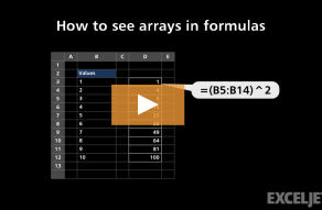
How to see arrays in formulas
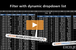
Filter with dynamic dropdown list

Spilling and the spill range

Unique values with criteria

How to count unique values
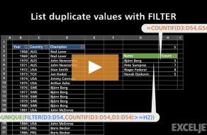
List duplicate values with FILTER
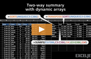
Two-way summary with dynamic arrays

New dynamic array functions in Excel

The UNIQUE function
Related functions

UNIQUE Function

FILTER Function
The Excel FILTER function is used to extract matching values from data based on one or more conditions. The output from FILTER is dynamic. If source data or criteria change, FILTER will return a new set of results. This makes FILTER a flexible way to isolate and inspect data without altering the...

SORT Function
The Excel SORT function sorts the contents of a range or array in ascending or descending order. Values can be sorted by one or more columns. SORT returns a dynamic array of results.

SORTBY Function
The Excel SORTBY function sorts the contents of a range or array based on the values from another range or array. The range or array used to sort does not need to appear in results.

RANDARRAY Function
The Excel RANDARRAY function generates an array of random numbers between two values. The size or the array is specified by rows and columns arguments. The generated values can be either decimals or whole numbers.

SEQUENCE Function
The Excel SEQUENCE function generates a list of sequential numbers in an array. The array can be one dimensional, or two-dimensional, determined by rows and columns arguments.


