Count cells that contain formulas

In this example, the goal is to count the number of cells in a range that contain formulas. This problem can be solved with a formula based on the SUMPRODUCT and ISFORMULA functions, as explained below.

Forecast values

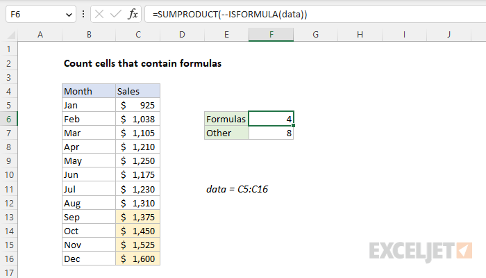
The values in the range C13:C16 are forecasts created with a formula based on the MROUND function. The formula in C13, copied down, is:

=MROUND(C12*1.05,25)

This formula generates values that are 5% higher than the previous month, rounded to the nearest multiple of 25.

ISFORMULA function

The ISFORMULA function returns TRUE if a cell contains a formula, and FALSE if not. For example, if cell A1 contains the =1+1 the following formula will return TRUE:

=ISFORMULA(A1) // returns TRUE

if cell A1 contains the the number 2 (hardcoded), ISFORMULA will return FALSE:

=ISFORMULA(A1) // returns FALSE

Count cells with formulas

In the worksheet shown, the range C5:C16 is named "data". To count cells in this range that contain formulas, the formula in cell F6 is:

=SUMPRODUCT(--ISFORMULA(data))

Working from the inside out, the ISFORMULA function checks all cells in data with this formula:

ISFORMULA(data)

Because there are 12 cells in the range, ISFORMULA returns 12 results in an array like this:

{FALSE;FALSE;FALSE;FALSE;FALSE;FALSE;FALSE;FALSE;TRUE;TRUE;TRUE;TRUE}

The FALSE values in this array represent cells that do not contain a formula. Each TRUE value represents a cell that does contain a formula. Notice the last 4 values are TRUE, which makes sense because these cells are forecast values created with a formula. The next step is to convert the TRUE and FALSE values to 1s and 0s. We do this with a double negative (--) operation:

--{FALSE;FALSE;FALSE;FALSE;FALSE;FALSE;FALSE;FALSE;TRUE;TRUE;TRUE;TRUE}

The result is a numeric array that contains only 1s and 0s:

{0;0;0;0;0;0;0;0;1;1;1;1}

This array is delivered directly to the SUMPRODUCT function:

=SUMPRODUCT({0;0;0;0;0;0;0;0;1;1;1;1}) // returns 4

With only one array to process, SUMPRODUCT simply sums the array and returns a final result of 4.

Not formulas

To count cells in data that do not contain formulas, you can add the NOT function like so:

=SUMPRODUCT(--NOT(ISFORMULA(data)))

This is the formula in cell F7. The NOT function reverses the TRUE FALSE results returned by the ISFORMULA function, and returns the resulting array directly to SUMPRODUCT:

=SUMPRODUCT({1;1;1;1;1;1;1;1;0;0;0;0}) // returns 8

As before, SUMPRODUCT sums the values in the array and returns a result of 8.

Note: in the dynamic array version of Excel, you can use the SUM function instead of the SUMPRODUCT function with the same result. To learn more about why this topic, see Why SUMPRODUCT?