Summary
If you need to perform multiple lookups sequentially, based on whether the earlier lookups succeed or not, you can chain one or more VLOOKUPs together with IFERROR.
In the example shown, the formula in L5 is:
=IFERROR(VLOOKUP(K5,B5:C7,2,0),IFERROR(VLOOKUP(K5,E5:F7,2,0),VLOOKUP(K5,H5:I7,2,0)))
Generic formula
=IFERROR(VLOOKUP 1,IFERROR(VLOOKUP 2,VLOOKUP 3))
Explanation
The IFERROR function is designed to trap errors and perform an alternate action when an error is detected. The VLOOKUP function will throw an #N/A error when a value isn't found.
By nesting multiple VLOOKUPs inside the IFERROR function, the formula allows for sequential lookups. If the first VLOOKUP fails, IFERROR catches the error and runs another VLOOKUP. If the second VLOOKUP fails, IFERROR catches the error and runs another VLOOKUP, and so on.