Hey, Dave here from Exceljet.
We recently did a survey and asked people what they wanted to learn most about Excel formulas and functions. One of the most popular replies was logical functions: formulas that use IF, sometimes with OR, sometimes with AND.
So I thought I would do some training that shows you how to build up logical formulas.
I'll start at the beginning with some logical expressions that evaluate to TRUE and FALSE. Then I'll look at how you combine those using the OR function for an OR relationship, and the AND function for an AND relationship.
Finally, we'll put that into an IF function, so you can test a condition and take one action if the result is TRUE, and a different action if the result is FALSE.
Let's go to the training.
Okay, here we are in Excel, and I'm going to enter some simple logical statements that return either TRUE or FALSE. These kinds of statements are the building blocks for more complex formulas that do more advanced conditional analysis.
In the first case, we're going to test the cells in column B to see if they equal 80. To do that, we type an equal sign, B5, and then equal 80:
=B5=80
It's a very simple formula. When I hit return, we get FALSE, because 69 is not 80. And when I copy that down, we get FALSE everywhere except for the last value, because cell B10 is 80.
For "not 80", we start again with equals and B5, and we use the "not equal to" operator, which is just the less than and greater than symbols together:
=B5<>80
When I copy this down, you'll see we get the mirror image of the values in column C. Now the only FALSE value is the last one.
Greater than 80 is B5, a greater than sign, and 80:
=B5>80
Copy that down, and we only get TRUE where we have a value greater than 80.
If you need greater than or equal to 80, we add an equal sign after the greater than sign:
=B5>=80
When we copy that down, we get the same values, except the last one in F10 is TRUE, because the value in B10 is 80.
For text, you'll need to wrap the text in double quotes. So, to test for the color green, the formula is H5 equals "green" in quotes:
=H5="green"
We only get TRUE in I7, because H7 is green.
For "not green", we use the "not equal to" operator again, with green in double quotes:
=H5<>"green"
When we copy this down, we get TRUE everywhere except in J7.
Okay, now we're going to look at how to combine logical statements using the AND function and the OR function.
In the first case, we want to return TRUE if a value is between 75 and 90. This is an AND relationship, so we type equals, AND, and open the parentheses. You can see we need to provide logical1, and logical1 is B5 is greater than 75. Then a comma, and now we're at logical2, which is B5 is less than 90:
=AND(B5>75,B5<90)
When I hit enter and copy that down, you can see that we're now correctly testing for values that are between 75 and 90.
The other relationship you may want to use with logical statements is OR, and for that you use the OR function. We start off with equals, OR, and when I open the parentheses, we're at logical1. Logical1 is for the color green, so we type E5 equals "green". Then a comma, and logical2 is E5 equals "red":
=OR(E5="green",E5="red")
Now this formula is testing for colors that are either green or red.
Finally, let's look at how to combine the OR and AND functions together. In this case, we want to test for the color red or green, and a quantity greater than 10.
We start off with AND, and right away we go to an OR, because we're testing two colors. That's H5 equals "red", and H5 equals "green". Close the parentheses, and when we type a comma, we're on the second logical for AND. The first logical was the OR formula, and the next one is quantity greater than 10:
=AND(OR(H5="red",H5="green"),I5>10)
When we copy this down, we get TRUE only when the color is red or green and the quantity is greater than 10.
Okay, now let's look at how to combine these logical statements inside the IF function.
In this case, a passing score is greater than 80. We know how to test for that now; it's just C5 greater than 80:
=C5>80
We hit return and get FALSE, because 69 is not greater than 80, and you can see that everybody passed but Sarah and Tim.
Now, if you want to display a message, we type equals IF to start the IF function, and we put in the same test, C5 greater than 80. For value_if_true we'll use "Pass", and for value_if_false we'll use "Fail":
=IF(C5>80,"Pass","Fail")
When I copy that down, you'll see that we get a pass or fail for each score.
And if you don't want to display a value in some cases, let's say we want to show pass but not fail, we can get rid of the text for value_if_false. We have to put something there, so we'll put empty quotes, which means an empty string, which displays nothing:
=IF(C5>80,"Pass","")
When I hit return, you'll see we get nothing there, but we do get a pass in cases where the test score is greater than 80.
Now let's look at how to combine the IF function with the OR function. In this case, we have a list of employees, and we want to put employees in the Sales or Marketing department in group A, and employees in the other departments (Fulfillment, Support, and Engineering) in group B.
We'll start off with IF, and to keep it simple, let's just test for Sales. So, if F5 equals "sales", we'll put "A" for group A, and just leave it at that:
=IF(F5="sales","A")
We get FALSE in that case, but you can see we get the A's where the department is Sales.
Now let's extend that formula. I'm going to leave everything selected, cut the logical test out, put the OR function in, and paste. That's our first logical. The second one is F5 equals "marketing". Close the parentheses, and now I'm going to hit Control + Enter to update all the formulas:
=IF(OR(F5="sales",F5="marketing"),"A")
Now we have more A's, because we're correctly grouping Marketing as well.
Finally, to add the B group, all we need to do is provide a value_if_false. I'll backspace, provide "B" for value_if_false, and hit Control + Enter again:
=IF(OR(F5="sales",F5="marketing"),"A","B")
Now you can see that we have A's for Sales and Marketing and B for everything else.
In our last example, we're going to look at how to combine the IF function with the AND function. In this case, we have a list of properties, and we want to mark properties that have at least three bedrooms, less than 3000 square feet, and were built after 1979.
We'll start off with IF, and then we use AND, because all of these criteria are joined with an AND relationship.
First, we look for bedrooms, which is D5 greater than or equal to 3. For the next logical, we look for square footage, which is F5 less than 3000. And for logical3, we want properties built after 1979, which is G5 greater than 1979.
I close the parentheses, and we're done with the AND function. When I type a comma, we're on value_if_true. In this case, we'll use an "x" in quotation marks, which just displays text. For value_if_false, we'll display nothing, so we put double quotes, and close up the formula:
=IF(AND(D5>=3,F5<3000,G5>1979),"x","")
When I copy this down, you'll see that we're only marking properties that meet all three criteria.
Don't forget that you can use the screen tip window to navigate the different arguments. If we go up into the formula and click the IF function, you'll see that we can select the logical test right here, and notice that it is the entire AND function with all three criteria. We can also select value_if_true and value_if_false.
All right, I hope you enjoyed that training on logical formulas in Excel.