Summary
To calculate how long it will take to reach a savings goal with a fixed monthly amount, you can use the NPER function with a monthly rate. In the example shown, the formula in C12 is:
=NPER(C7/12,C6,C8,-C5)
where C5 contains the savings goal, C6 the monthly savings, C7 the expected annual return, and C8 the starting balance. With a goal of $60,000, monthly savings of $500, a 5% annual return, and $10,000 already saved, NPER returns 78.26 months, or about 6.5 years. See below for details, and for a check with the FV function.
Generic formula
=NPER(rate/12,monthly,start,-goal)
Explanation
"How long will it take to reach my savings goal?" is the natural follow-up to "how much do I need to save each month?", and Excel answers it with the NPER function. NPER returns the number of periods needed for an investment (or a loan) given a rate, a periodic payment, a present value, and a future value. In financial formulas, a period is a regular unit of time used to calculate interest, investment returns, or payment schedules, such as a year, a quarter, or a month. In this example, the period is a month. For a savings plan, the payment is the monthly deposit, the present value is what you have already saved, and the future value is the goal. NPER then tells you how many months it will take to get there. This page is the companion to Monthly savings needed to reach goal, which solves the same problem in the other direction with the PMT function.
In this example, the goal is to calculate how long it will take to reach $60,000 by saving $500 per month, assuming a 5% annual return and a starting balance of $10,000. The worksheet uses monthly periods throughout: the annual return is divided by 12 to get a monthly rate, and NPER returns a number of months, which is then converted to years. Online calculators often label the monthly amount the monthly deposit or monthly contribution; on this page it is called monthly savings.
Table of contents
- Worksheet setup
- The NPER formula
- Months, years, and rounding
- Managing the signs
- Checking the result with FV
- How to use this worksheet
- Saving more shortens the time
- Summary
Worksheet setup
The worksheet has four inputs in the range C5:C8 and three outputs in the range C12:C14:
| Input | Description | Example |
|---|---|---|
| Savings goal | The amount you want to have at the end | $60,000 |
| Monthly savings | The amount you will save each month | $500 |
| Annual return | The rate you expect the savings to earn each year | 5% |
| Starting balance | What you have saved already (enter 0 if nothing) | $10,000 |
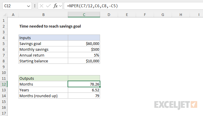
The main output is the number of months in C12, explained below. The other two outputs convert the result into more useful forms: years in C13, and whole months in C14. Both are covered in Months, years, and rounding.
The NPER formula
The formula in C12 is:
=NPER(C7/12,C6,C8,-C5)
The arguments are configured like this:
- rate is the annual return in C7 divided by 12, which gives a monthly rate of about 0.417%.
- pmt is the monthly savings in C6, $500.
- pv is the starting balance in C8, $10,000.
- fv is the savings goal in C5, entered as a negative number.
With these inputs, NPER returns 78.26. Since the rate is a monthly rate and the payment is a monthly amount, the result is a number of months. In other words, if you already have $10,000, and you save $500 at the end of every month while earning 5% per year, you will reach $60,000 a little more than 78 months from now. The starting balance and the monthly savings are entered as positive numbers, and the goal as a negative number, so that NPER returns a positive result. See Managing the signs below.
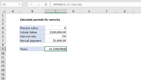
As with the other financial functions, the rate argument must match the payment period. Because the deposits are monthly, the annual return is divided by 12. If you save yearly instead, use the annual return as is and the yearly amount for pmt, and NPER will return a number of years. See Calculate periods for annuity for an example with annual payments.
Months, years, and rounding
NPER returns a fractional number of periods, which is precise but not very readable. The formula in C13 converts months to years:
=C12/12
which returns 6.52, so the goal is about six and a half years away. Since you can't make a fraction of a deposit, it is also useful to know the number of whole months. The formula in C14 uses the ROUNDUP function to round up to the next whole month:
=ROUNDUP(C12,0)
The result is 79. After 78 deposits the balance is still just short of the goal, and the 79th deposit takes it over. Always round up here, since rounding to the nearest month (78) would leave you short. To show the result as years and months, you can combine the INT function and the MOD function:
=INT(C14/12)&" years, "&MOD(C14,12)&" months" // returns "6 years, 7 months"
Managing the signs
Excel's financial functions use the sign of a number (+ or -) to show the direction the money is moving. The sign shows the direction of the money, not whether it is good or bad. Amounts that flow one way get one sign, and amounts that flow the other way get the opposite sign. Which direction is positive is up to you, as long as you are consistent. In this worksheet, the starting balance and the monthly savings both flow into the account, so they share a sign, and the goal flows out at the end, so it gets the opposite sign. The formula in C12 makes the goal negative to follow that convention.
Unlike PMT, NPER returns a count of months, and a count has no direction. This means you can reverse the signs and get the same result:
=NPER(C7/12,-C6,-C8,C5) // returns 78.26
What matters is that the goal has the opposite sign from the starting balance and the monthly savings. If all three share a sign, NPER returns the #NUM! error, because no number of months gets there. The same convention is explained on the Monthly savings needed to reach goal page.
Checking the result with FV
A good way to check the result is to work the problem in reverse with the FV function, which returns the future value of an investment given a rate, a number of periods, a periodic payment, and a present value. If the number of months is right, FV should return the goal. In the worksheet below, the inputs are the same as before, and the formula in C13 is:
=FV(C7/12,C12,-C6,-C8)
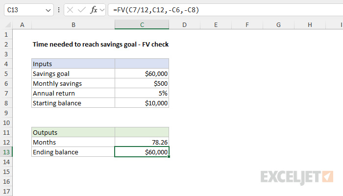
The rate is 5% divided by 12, the number of periods is the months calculated by NPER in C12, the payment is the monthly savings in C6, and the present value is the starting balance in C8. The payment and present value are entered as negative numbers (money paid in), so that FV returns a positive number. The result is $60,000, the savings goal, which confirms the result from NPER. Note that FV accepts a fractional number of periods, so the check works with the unrounded result from NPER.
How to use this worksheet
The worksheet is set up as a small calculator, so you can download it and enter your own numbers:
- Enter your savings goal in C5, the amount you plan to save each month in C6, the annual return you expect in C7, and what you have saved already in C8. Enter 0 in C8 if you are starting from scratch.
- Read the result in C12 (months), C13 (years), and C14 (whole months, rounded up). The number in C14 is the number of deposits you will actually make.
- Try a few what-ifs by changing the inputs. Each change updates the outputs right away.
Some what-ifs worth trying with the example inputs:
- Starting balance of 0. With nothing saved yet, NPER returns 97.51 months, a little over 8 years, instead of 78.26.
- Return of 0%. With no growth, the time to the goal is just the gap between the goal and the starting balance divided by the monthly savings, and NPER returns exactly 100 months. This is a useful sanity check: any positive return should give a smaller number.
- A larger monthly amount. The table in the next section shows how the time drops as the monthly savings go up.
The only variation that needs a formula change is the timing of the deposits. By default, NPER assumes each payment is made at the end of the period. If you deposit at the start of each month, each deposit earns one extra month of return, and the goal arrives slightly sooner. To model this, set the optional type argument to 1:
=NPER(C7/12,C6,C8,-C5,1) // returns 78.01
Finally, there are two other NPER behaviors you should know about: if the starting balance is already larger than the goal, NPER returns a negative number, and if both the starting balance and the monthly savings are zero, NPER returns #NUM!, since a balance of zero never grows.
Saving more shortens the time
The table below shows the time to reach $60,000 with $10,000 already saved at a 5% return, for several monthly amounts:
| Monthly savings | Months | Years |
|---|---|---|
| $250 | 129.6 | 10.8 |
| $500 | 78.3 | 6.5 |
| $750 | 56.2 | 4.7 |
| $1,000 | 43.8 | 3.7 |
| $1,500 | 30.5 | 2.5 |
Notice that doubling the monthly amount from $500 to $1,000 cuts the time from 78 months to 44, less than half. That is because the starting balance and the return do a fixed share of the work no matter how much you save, so extra savings have a smaller effect on the total. Over longer periods, the return rate matters more. At a 7% return, the $500 plan reaches the goal in about 6.0 years instead of 6.5.
This worksheet is a planning estimate only, not a guarantee. Unless you are investing in a fixed-rate investment like a Treasury or a CD, the return rate is an assumption only and will vary. Also, remember the formulas do not account for taxes, fees, or inflation.
Summary
The NPER function calculates the time needed to reach a savings goal:
- Divide the annual return by 12 for the rate argument so that the result is in months, then divide by 12 to convert to years.
- Enter the monthly savings as pmt, the starting balance as pv, and the goal as a negative fv. Use 0 for pv if you are starting from scratch.
- Round the result up with ROUNDUP to get the number of deposits actually needed.
- Check the result with the FV function: the same rate, the months from NPER, and the monthly savings and starting balance as negative numbers, should return the goal.
- Set type to 1 if deposits are made at the start of each month.
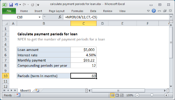
To go the other way and calculate the monthly amount needed to reach a goal by a set date, see Monthly savings needed to reach goal. For the number of payments needed to pay off a loan, see Calculate payment periods for loan.