Summarize weather data by day and month

Summary

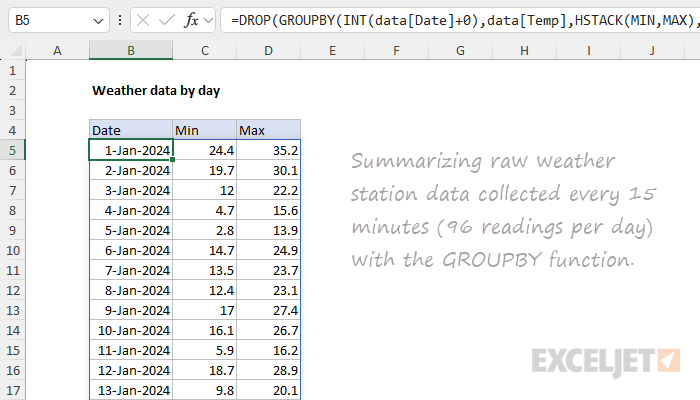
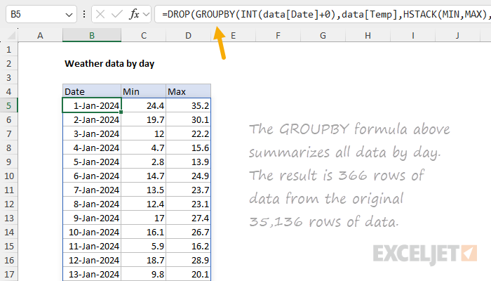
To summarize granular weather station data by day, you can use the GROUPBY function together with a few helper functions. In the worksheet shown, the source data is in an Excel Table named data on the data sheet, with one reading every 15 minutes for all of 2024. The formula in cell B5 of the day sheet returns the minimum and maximum temperature for each day:

=DROP(GROUPBY(INT(data[Date]+0),data[Temp],HSTACK(MIN,MAX),,0,,data[Temp]<>""),1)

The result spills into a clean three-column array: date, daily min, daily max. Building on top of the daily summary, a second formula on the month sheet rolls the data up by month and adds the date on which each month's minimum and maximum occurred. See the Explanation below for a full walkthrough of both formulas.

Most weather stations record many fields: temperature, humidity, wind speed and direction, barometric pressure, rainfall, solar radiation, and so on. To keep this example simple, the workbook includes just a few columns, and we only summarize the temperature column. The same techniques will work with other measurement data.

Explanation

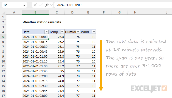
In this example, the goal is to summarize a year of granular weather station readings (about 35,000 rows, one every 15 minutes) into a daily summary, then a monthly summary. The daily summary is a single GROUPBY formula. The monthly summary is more involved because, in addition to the monthly min and max temperatures, we also want the date on which each min and max occurred. To get those dates, we'll use MAP, LAMBDA, and XLOOKUP inside a LET formula.

This is a surprisingly challenging problem in Excel and a good example of how Excel's new dynamic array formulas can really help. Read below for details. There are a few useful tricks along the way.

The source data
Summary by day
Summary by month
Final thoughts

The source data

The source data is in an Excel Table named data on the data sheet, with one reading every 15 minutes for all of 2024. That works out to roughly 35,000 rows. The table has four columns: Date, Temp, Humidity, and Wind. Temperatures are in degrees Fahrenheit. The Date column carries a full datetime value (date plus time of day), which is what allows multiple rows per day.

The data in the workbook is synthetic, modeled on actual 2024 weather for Chicago, Illinois. It's representative of what a real weather station would record, but it's not the real readings.

Raw weather station data in an Excel Table named 'data', with a reading every 15 minutes

Because the data lives in an Excel Table, the formulas below stay dynamic. If new readings are added to the table, the daily and monthly summaries will recalculate automatically.

Summary by day

The daily summary lives on the day sheet. The formula in cell B5 spills a three-column array: date, minimum temperature for that day, and maximum temperature for that day:

=DROP(GROUPBY(INT(data[Date]+0),data[Temp],HSTACK(MIN,MAX),,0,,data[Temp]<>""),1)

Daily summary spilled from a single GROUPBY formula, with date, min temp, and max temp columns

There are a few things to notice here.

Stripping the time off the date. GROUPBY needs to group by day, but the Date column carries a full datetime value, so each timestamp is unique. To collapse the timestamps to a date, we wrap the column with INT, which discards the fractional part of an Excel datetime and leaves just the integer date. (For more on this pattern, see Remove time from timestamp.)

=INT(data[Date]+0)

What's the +0 doing? In this workbook, the values in the Date column are actually text, not real Excel dates. (This is typical when raw weather data is dumped to CSV and opened in Excel without any conversion.) Adding 0 forces Excel to coerce the text into a real serial date number, which INT can then truncate. Without the +0, INT would error on the text values. If your Date column already contains real dates, you can drop the +0 and use plain INT(data[Date]), but adding zero does no harm.

Two aggregations at once. GROUPBY's function argument accepts a single function like SUM or AVERAGE, but it also accepts an array of functions. Stacking them with HSTACK tells GROUPBY to apply both:

HSTACK(MIN,MAX)

The result is two output columns, one for each function, in the order given.

Filtering out empty readings. The last argument is GROUPBY's filter_array, which restricts the calculation to rows that meet a condition. We use it to skip any timestamps where the Temp column is empty:

data[Temp]<>""

Weather stations sometimes go offline and generate empty results during a short time period, so this step is a guard against rows that might not have real data.

Why DROP? When function is an array (as it is here), GROUPBY automatically adds a header row at the top of the output labeled with the function names ("MIN", "MAX"). We are adding our own headers manually, so we don't want this header in the spilled result. Using DROP with 1 is a clean way to remove only the first (header) row:

=DROP(GROUPBY(...),1)

The final result is the daily summary. One formula spills 366 rows (2024 was a leap year), with no helper columns.

Summary by month

The monthly summary lives on the month sheet. The formula in cell B5 spills a five-column array: month, min temp, max temp, date of the min, and date of the max.

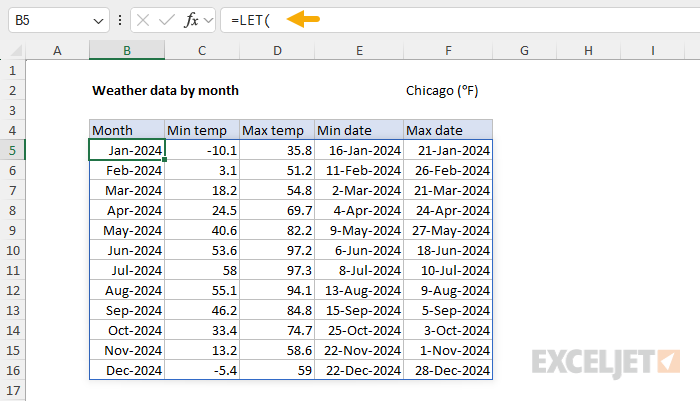
Monthly summary with month, min temp, max temp, date of min, and date of max columns

The interesting columns are the last two. Knowing that the coldest temperature in January was -10.1°F is useful, but it's more useful to also know it happened on January 16. Finding that date requires a bit of work because GROUPBY can summarize values, but it can't easily tell you where a value came from. Here's the full formula in cell B5:

=LET(
    day_data,day!B5#,
    day_date,CHOOSECOLS(day_data,1),
    day_min,CHOOSECOLS(day_data,2),
    day_max,CHOOSECOLS(day_data,3),
    result,DROP(GROUPBY(EOMONTH(day_date,-1)+1,HSTACK(day_min,day_max),HSTACK(MIN,MAX),,0),1),
    months,CHOOSECOLS(result,1),
    min_temps,CHOOSECOLS(result,2),
    max_temps,CHOOSECOLS(result,3),
    min_dates,MAP(months,min_temps,LAMBDA(m,t,XLOOKUP(1,(day_min=t)*(TEXT(day_date,"mmyy")=TEXT(m,"mmyy")),day_date))),
    max_dates,MAP(months,max_temps,LAMBDA(m,t,XLOOKUP(1,(day_max=t)*(TEXT(day_date,"mmyy")=TEXT(m,"mmyy")),day_date))),
    HSTACK(result,min_dates,max_dates)
)

It looks like a lot, but don't panic. Every line is doing one small job. Let's go through the formula step by step.

Pulling in the daily summary

The monthly summary is built on top of the daily summary, not on the raw 35,136-row data. Working from the daily summary makes the formula faster and easier to understand. The reference day!B5# is the spilled range operator: it grabs the entire spilled array that starts at day!B5, no matter how many rows it contains. We assign it to a LET variable named day_data so we can reuse it without repeating the reference, and then we split it into three named columns using CHOOSECOLS:

day_data,day!B5#,
day_date,CHOOSECOLS(day_data,1),
day_min,CHOOSECOLS(day_data,2),
day_max,CHOOSECOLS(day_data,3),

Now day_date, day_min, and day_max are three parallel one-column arrays we can refer to by name in the rest of the formula. Importantly, all three names trace back to the spill reference, which means they will automatically resize to track changes in the data.

Grouping by month

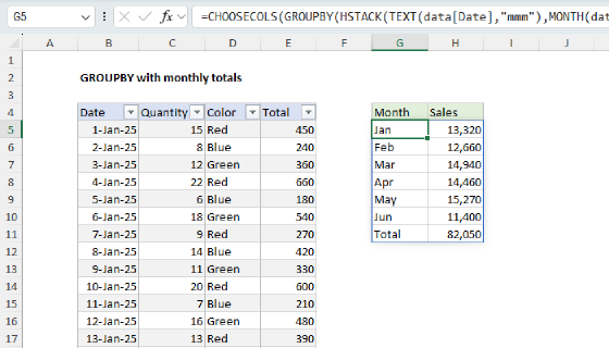
The monthly grouping uses the same trick as in GROUPBY with monthly totals: instead of converting dates to month names (which sort alphabetically) we remap each daily date to the first day of its month, then let GROUPBY group on those dates. The first-of-month dates sort chronologically without any extra effort:

EOMONTH(day_date,-1)+1

EOMONTH with -1 returns the last day of the previous month, and adding 1 lands us on the first day of the current month. (See Get first day of month for more on this pattern.)

The full GROUPBY call looks like this:

result,DROP(GROUPBY(EOMONTH(day_date,-1)+1,HSTACK(day_min,day_max),HSTACK(MIN,MAX),,0),1),

The values to aggregate are stacked with HSTACK so that GROUPBY can summarize the daily mins and maxes side by side. The function array is HSTACK(MIN,MAX), just like in the daily formula. Total_depth is set to 0 to suppress the totals row, and DROP trims the header row that GROUPBY adds when function is an array. The result is a three-column array: month, monthly min, monthly max.

Note that you can stop here if you want. If you don't care about the min and max dates, you can end the formula here and return result as a final value:

=LET(
    day_data,day!B5#,
    day_date,CHOOSECOLS(day_data,1),
    day_min,CHOOSECOLS(day_data,2),
    day_max,CHOOSECOLS(day_data,3),
    result,DROP(GROUPBY(EOMONTH(day_date,-1)+1,HSTACK(day_min,day_max),HSTACK(MIN,MAX),,0),1),
    result
)

Try it: edit the formula so that "result" is the last line in LET, on its own. The result will be a table with three columns only: Month, Min temp, and Max temp.

Finding the date of each min and max

This is the part that does most of the work. For each month, we want to find the date on which the monthly minimum (and maximum) occurred. The challenge is that we have to look across the daily summary to find that date, but only within the rows that belong to the current month.

First, we need some data to use in our lookups, some of which comes from the GROUPBY summary we just constructed. To start, we split the result into named columns the same way we did above:

months,CHOOSECOLS(result,1),
min_temps,CHOOSECOLS(result,2),
max_temps,CHOOSECOLS(result,3),

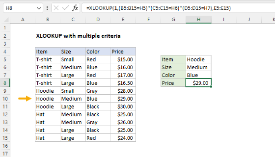
Next, we need to perform the actual lookups in the daily data in the "day" sheet. There are different ways we could do this in Excel, but XLOOKUP with Boolean logic is a pretty good approach. The pattern is to multiply two TRUE/FALSE conditions together and look up the result 1:

XLOOKUP(1,(day_min=t)*(TEXT(day_date,"mmyy")=TEXT(m,"mmyy")),day_date)

Here t is the monthly min temperature we're looking for, and m is the first-of-month date for that row. The first condition matches any day whose minimum equals t. The second condition restricts the match to the correct month. Multiplying TRUE/FALSE values produces 1 where both are true and 0 elsewhere, and XLOOKUP finds the first 1 and returns the corresponding date from day_date. (For more on this two-criteria pattern, see XLOOKUP with multiple criteria.)

Why use TEXT(...,"mmyy") for the month comparison instead of just comparing the dates directly? Because day_date carries the actual day of the month (January 1, January 2, January 3, ...) while m is always the first of the month. Comparing them directly only matches on the 1st of each month. Instead, we convert both dates to a "mmyy" text string ("0124" for January 2024) to collapse every day in a month to the same value, so any day in that month matches. In brief, this is a nice trick to quickly check if dates are in the same month and year while ignoring the actual day.

The XLOOKUP gives us one date for one month. To look up dates for every month at once, we wrap XLOOKUP in MAP and LAMBDA like this:

min_dates,MAP(months,min_temps,LAMBDA(m,t,XLOOKUP(1,(day_min=t)*(TEXT(day_date,"mmyy")=TEXT(m,"mmyy")),day_date))),

MAP "walks" months and min_temps in parallel and runs the LAMBDA once per row, with m set to the month and t set to that month's min temp. The result is a 12-row array of dates, one for each month.

The max_dates line does the same thing for the maximum:

max_dates,MAP(months,max_temps,LAMBDA(m,t,XLOOKUP(1,(day_max=t)*(TEXT(day_date,"mmyy")=TEXT(m,"mmyy")),day_date))),

Stacking the final result

At this point, we have a column of min dates and a column of max dates, but they are separate. The last line of the LET stitches everything together by stacking the original three-column GROUPBY result with the two new date columns:

HSTACK(result,min_dates,max_dates)

The final result generates five columns: month, min temp, max temp, min date, and max date. That's the spilled array you see in the worksheet starting in cell B5. The headers in row 4 are entered by hand and are not part of the output.

If two days in a month happen to record the exact same minimum (or maximum) temperature in the same month, the XLOOKUP returns the date of the first match.

Final thoughts

An interesting step in this example is building the monthly summary on top of the daily summary instead of on top of the raw data. The daily summary has already done the hard work of collapsing 35,000 rows down to 366, and that smaller dataset is easier to feed into the monthly formula. Plus, the daily summary displays useful information. The "find the date of the min/max" part of the monthly summary formula is quite complex. You could set up separate external formulas to do this work, but they also would be somewhat complex and redundant. Keeping everything together allows you to leverage the variables and values already defined in the formula. Let me know if you have a better approach!

Was this page helpful?

Author

Dave Bruns

Hi - I'm Dave Bruns, and I run Exceljet with my wife, Lisa. Our goal is to help you work faster in Excel. We create short videos, and clear examples of formulas, functions, pivot tables, conditional formatting, and charts.