Running balance with debits and credits

Summary

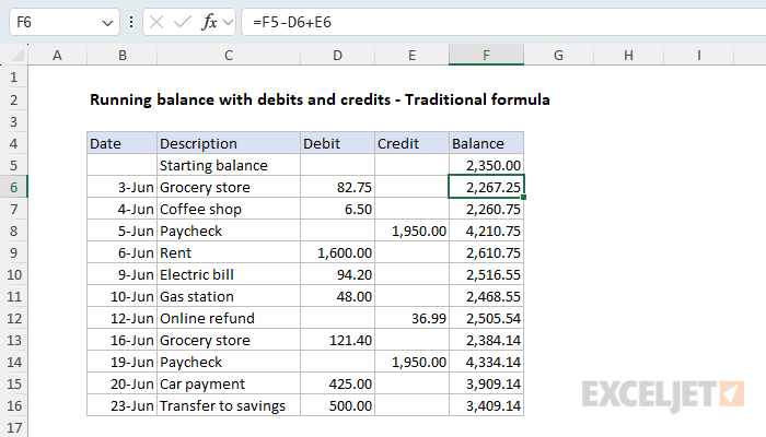
To calculate a running balance with debits and credits, you can use a simple formula that starts with the previous balance, subtracts debits, and adds credits. In the example shown, the formula in cell F6, copied down, is:

=F5-D6+E6

As the formula is copied down column F, it calculates a running balance in each row. This formula is easy to understand, but it breaks easily when rows are inserted or deleted.

See below for an alternative based on the SCAN function that calculates all balances with a single formula and handles inserted and deleted rows gracefully.

Generic formula

=balance-debit+credit

Explanation

In this example, the goal is to calculate a running balance for a list of transactions that includes both debits and credits. The worksheet follows the convention used on a bank statement: a debit is money leaving the account (a payment or withdrawal) and a credit is money coming into the account (a deposit or refund). Each transaction has a date and description, with amounts in the Debit column (D) or the Credit column (E). The starting balance appears in cell F5, and the goal is to calculate the balance after each transaction in column F. This is the same problem you would solve in a paper check register, and the same structure works for any transaction list with money in and money out.

The article below explains two approaches. The first is the traditional solution: a simple formula with relative addresses copied down the column. This formula is very basic, but it is surprisingly fragile when rows are inserted or deleted. The second approach uses the SCAN function to calculate every balance at once with a single formula. SCAN takes more effort to understand at first, but the result is simpler and more robust, and it is a nice example of how dynamic array formulas have changed the way even simple problems are solved in Excel.

Traditional formula
The problem with inserting and deleting rows
The SCAN alternative
Making the range dynamic
Which formula should you use?

Traditional formula

The classic way to calculate a running balance is to take the previous balance, subtract any debit, and add any credit. In the worksheet shown, the formula in cell F6, copied down, is:

=F5-D6+E6

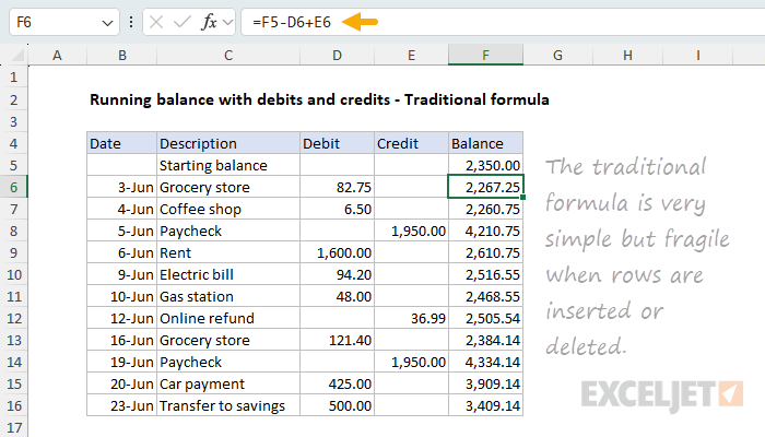
Running balance with a simple formula copied down

The formula picks up the balance in F5, then subtracts the value (if any) in D6 and adds the value (if any) in E6. When a debit or credit cell is empty, Excel treats it like zero, so it has no effect on the result. For example, the first transaction is a debit of $82.75 with no credit, so the formula returns 2350-82.75+0, which is $2,267.25.

Because the references are relative, the formula updates in each row as it is copied down: each balance is based on the balance directly above. This chain of simple formulas works fine in all versions of Excel, as long as the chain is never broken.

The problem with inserting and deleting rows

The weakness of the traditional formula is that every balance depends on the cell directly above. Inserting or deleting rows breaks the chain in different ways:

Inserting a row creates a gap. The new row has no formula, and the formula below it still refers to the old row above, skipping the new row entirely. To fix the problem, you need to copy the formula from a row above into the new row and the row below it.
Deleting a row is worse. The formula in the row below the deleted row loses the cell it refers to and returns the #REF! error, and every formula below that returns #REF! as well, since each balance depends on the one above. You can see this below, where the screenshot shows the effect of deleting row 12, which contained "Online refund":

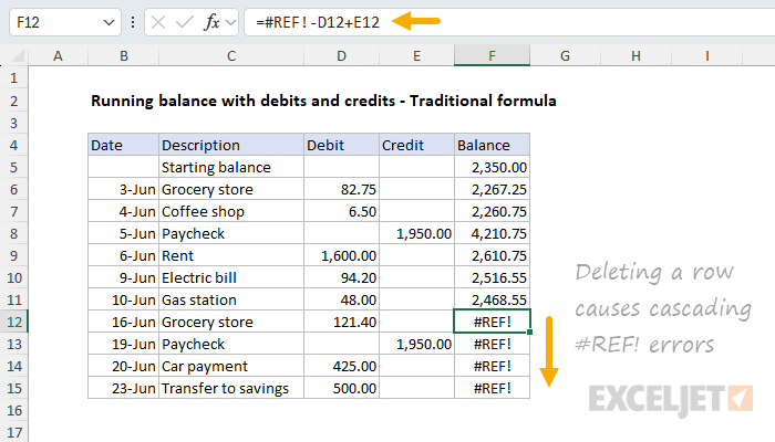
Deleting a row causes cascading #REF! errors

In short, the formula is somewhat fragile. The fix in both cases is the same: select a cell with a good formula above the problem, then copy the formula down through the rest of the column. This is not hard once you understand what is going on, but it often trips up beginners, and it means the worksheet formulas need repair whenever rows are deleted or inserted.

The SCAN alternative

The SCAN function solves the same problem with a single formula. In the worksheet below, the formula in cell F6 is:

=SCAN(F5,E6:E16-D6:D16,SUM)

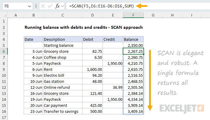
Running balance with a single SCAN formula

The result is the same set of balances as before, calculated all at once. The formula lives only in cell F6, and the results spill into the range F6:F16. There is nothing to copy down.

Working from the inside out, the expression E6:E16-D6:D16 subtracts each debit from each credit to calculate the net change for every transaction. As before, empty cells behave like zero. Because the ranges contain 11 rows, the result is an array with 11 net changes:

{-82.75;-6.5;1950;-1600;-94.2;-48;36.99;-121.4;1950;-425;-500}

Notice debits appear as negative numbers and credits appear as positive numbers after subtraction. This subtraction is the one tricky part of the formula: SCAN only accepts one array argument, so we need to combine the debits and credits into a single array. Subtracting debits from credits creates that array, and converts the debits to negative numbers so that we can use a sum operation to generate a running balance. The resulting array is delivered to SCAN as the array argument, with the starting balance in F5 as the initial_value.

SCAN moves through the array one value at a time, keeping a running "accumulator" that starts at the value in F5. At each new value, SCAN applies the SUM function, which sums the accumulator and the current net change, then updates the accumulator as it goes. The accumulator acts as the running balance and the behavior is exactly like the traditional formula, except that SCAN returns all intermediate balances in a single array:

{2267.25;2260.75;4210.75;2610.75;2516.55;2468.55;2505.54;2384.14;4334.14;3909.14;3409.14}

Note that passing SUM directly as the function is a compact shorthand. The more general way to write the same formula is with the LAMBDA function:

=SCAN(F5,E6:E16-D6:D16,LAMBDA(a,v,a+v))

In this version, a is the accumulator (the balance so far) and v is the value of the current net change. The calculation a+v adds the net change to the balance, the same operation SUM performs above. For more details on the abbreviated syntax and the long-hand LAMBDA, see our main SCAN page. To learn more about how arrays work in Excel formulas, see Arrays in Excel.

A key benefit of the SCAN formula appears when the transaction list changes. When you insert a row inside the range, Excel expands the references from E6:E16 to E6:E17 automatically, and the spilled results grow to match. When you delete a row, the references contract. Either way, SCAN recalculates the entire balance column instantly, with no gaps or #REF! errors.

Note: the SCAN function requires a current version of Excel and is available in Excel 2024+ and Excel 365. In older versions of Excel, use the traditional formula above.

Making the range dynamic

The SCAN formula above uses fixed ranges: E6:E16 and D6:D16. These references adjust when you insert or delete rows inside the range, but they will not pick up new transactions added at the bottom of the list. To make the running balance track the data automatically, you can use the TRIMRANGE function to trim a larger range down to the data it contains. In the worksheet below, the formula in cell F6 looks like this:

=LET(
  data,TRIMRANGE(D6:E1000),
  debits,INDEX(data,,1),
  credits,INDEX(data,,2),
  SCAN(F5,credits-debits,SUM)
)

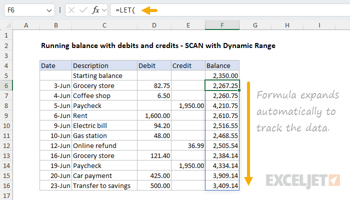
Running balance with SCAN and a dynamic range

The LET function keeps the formula readable by naming each part. The key step is to create a dynamic range that automatically tracks the data with the TRIMRANGE function like this:

data,TRIMRANGE(D6:E1000) // create dynamic range

TRIMRANGE removes the empty rows below the last transaction, so data ends at the last row that contains a debit or a credit. The INDEX function then splits data into debits (column 1) and credits (column 2). Notice the row_num argument in INDEX is omitted, which tells INDEX to return the entire column. Finally, SCAN calculates the running balance as before. Now when new transactions are added below row 16, the formula picks them up automatically and returns a balance for every row.

The Debit and Credit columns cannot be trimmed separately, because they may not end on the same row. As a more concise alternative to TRIMRANGE, you can use the dot operator: the expression D6:.E1000 performs the same trim operation. E1000 is an arbitrary limit; use a number that makes sense for your use case. Note that TRIMRANGE and the dot operator are currently available in Excel 365 only.

You might expect an Excel Table to be a natural way to solve this problem, since tables grow automatically as new data is added. However, the SCAN formula will not work inside an Excel Table, because dynamic array formulas cannot spill inside a table. This is a key limitation of dynamic array formulas at present.

Which formula should you use?

If you learned Excel before dynamic arrays, the traditional formula is probably the solution you reach for first, and it remains a fine choice: it is easy to write, easy to understand, and works in every version of Excel. Just remember that inserting and deleting rows will break the chain, so you will need to re-copy formulas as needed.

The SCAN formula is a good example of the trade-off that comes with many dynamic array formulas: more effort to understand up front, but a simpler and more robust result in the end. Key points:

The traditional formula =F5-D6+E6 must be copied down, and must be repaired after rows are inserted or deleted
The SCAN formula calculates all balances at once and spills the results into the balance column
SCAN expands and contracts automatically when rows are inserted or deleted inside the range, and can be configured with a dynamic range to track new transactions
SCAN requires Excel 2024+ or Excel 365

I would probably use the SCAN formula on a new worksheet when all users have a current version of Excel. But for teaching how Excel cell references work, the traditional formula is a better starting point.