Summary
To match and summarize noisy data in Excel, where the same value appears in many different forms, you can use a map table together with the XLOOKUP function and the GROUPBY function. In the example shown, the formula in cell F5 is:
=GROUPBY(XLOOKUP(data[Country],map[Input],map[Output]),data[Sales],SUM)
where data is an Excel Table containing noisy country names and sales values, and map is a small Excel Table that maps each variation to a clean name. The result is a clean summary of total sales by country, even though the underlying data contains 21 different spellings of just 4 countries.
Generic formula
=GROUPBY(XLOOKUP(data,map_in,map_out),values,SUM)
Explanation
In this example, the goal is to summarize sales by country using the data shown below. There is just one problem: the country names are a complete mess. The first three rows alone contain "USA", "United States", and "Germany", and as you scroll down you'll find variations like "U.S.A.", "America", "US", "Deutschland", "DEU", "GER", "DE", "Great Britain", "England", "GBR", "Frankreich", "FR", and "FRA". In total, there are 21 different spellings for just 4 countries. Trying to summarize this data with a Pivot Table or a GROUPBY formula on the raw country column would give us 21 separate rows instead of 4. Before we can summarize anything, we need a way to collapse all of these variations down to a single clean name per country. The article below explains how to do this with a lookup formula and a map table, and how to use another formula to flag new names that need to be added to the map.
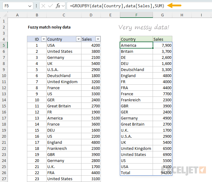
Table of contents
- Dave, this isn't fuzzy matching!
- The map table
- Looking up a clean name with XLOOKUP
- Summarizing with GROUPBY
- Finding missing inputs
- Why a map table is a good solution
- Formula for older versions of Excel
- Final thoughts
Dave, this isn't fuzzy matching!
Yes, I know :) I'm just using the word "fuzzy" because that's what most people call this kind of problem, and what people search for when they run into a challenge like this. The technique below isn't fuzzy matching in the strict sense (true fuzzy matching wouldn't help much here anyway), but it solves the same problem more reliably.
A couple of things to keep in mind:
- Excel does not have a built-in fuzzy match function. There is no FUZZYMATCH or FUZZYLOOKUP. Most fuzzy matching in Excel is done in Power Query, with custom functions, or with VBA.
- Even if Excel did have a fuzzy match function, it wouldn't solve this problem. Fuzzy matching algorithms (like Levenshtein distance) measure how similar two strings are. They work well when the variation is small: typos, extra spaces, different capitalization, etc. They do not work well when "USA", "America", "US", and "United States" all need to map to the same value.
The map table
The core of the solution is a small two-column Excel Table called map that lists every variation we expect to see in the data and the clean name we want it mapped to. The first column is Input (the noisy value that appears in the source data), and the second column is Output (the clean value we want to use in our summary).
The Missing Inputs table shows unmapped values in the source data. See explanation below.
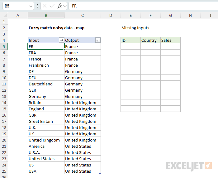
For example:
| Input | Output |
|---|---|
| FR | France |
| FRA | France |
| France | France |
| Frankreich | France |
| DE | Germany |
| DEU | Germany |
| Deutschland | Germany |
| GER | Germany |
| Germany | Germany |
| ... | ... |
Building the map table is the hardest part of this technique. You need to look at the data, identify each unique variation, and decide what the clean name should be. The good news is that this is a one-time effort. Here are the steps:
- Use the UNIQUE function to extract all distinct values from the source column with a formula like
=UNIQUE(data[Country]). This gives you a clean list of every variation that appears in the data. (In an older version of Excel, you can use Advanced Filter to get a list of unique values.) - Copy the spilled result and paste it back as values (Ctrl + Shift + V) in a new location. This step is necessary because dynamic array formulas like UNIQUE cannot be used inside an Excel Table, so we need static values for the next step.
- Convert the values into an Excel Table (Ctrl + T) with two columns: Input and Output. Initially, the Output column will be empty.
- Fill in the Output column with the clean name for each Input.
- Sort the table by the Output column first, then by the Input column. This brings related variations together, so all the "United States" inputs sit in one block, all the "Germany" inputs sit in another, and so on. Sorting this way makes it much easier to spot mistakes and to see at a glance how each clean name is being mapped.
Building the map table is also a good use case for AI. AI can scan a column of noisy data, identify the unique values, and propose a clean name for each. Drop the result into an Excel Table. But building the table manually will give you a better understanding of the data.
Looking up a clean name with XLOOKUP
Once the map table exists, replacing each noisy value with its clean name is a straightforward XLOOKUP operation. The basic idea is to look up each value in the Country column of the source data inside the Input column of the map, and return the matching value from the Output column:
=XLOOKUP(data[Country],map[Input],map[Output])
- The lookup_value is
data[Country], the entire column of noisy country names from the source table. - The lookup_array is
map[Input], the column of variations in the map table. - The return_array is
map[Output], the column of clean names.
Because we pass an entire column to XLOOKUP as the lookup_value, this is an array operation. XLOOKUP returns a clean country name for every row in the source data. If we entered this formula on its own in a worksheet cell, it would spill down with one clean country name per row of source data.
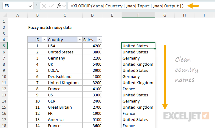
Notice we don't need a match_mode argument because XLOOKUP performs an exact match by default. This is what we want: the map table is the source of truth, and every input should match cleanly.
Summarizing with GROUPBY
The XLOOKUP above gives us the normalized values, but the real goal is to summarize those values. To get a total per country, we wrap the XLOOKUP inside GROUPBY:
=GROUPBY(XLOOKUP(data[Country],map[Input],map[Output]),data[Sales],SUM)
- The row_fields argument is the result from XLOOKUP, the array of clean country names.
- The values argument is
data[Sales], the sales numbers we want to add up. - The function argument is SUM, because we want a total per country.
The result is a clean summary table with one row per country, plus a total row, all from a single formula:
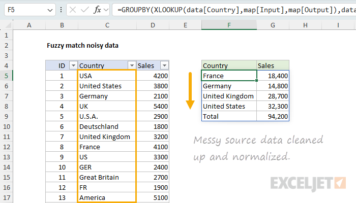
What's nice about this approach is that the XLOOKUP and GROUPBY do all the work in a single formula. There is no helper column on the source data, no Pivot Table to refresh, and no manual cleanup. If a sales number changes, or a row is added to the source table, the summary updates immediately.
Finding missing inputs
A map table only works if it covers every value that appears in the source data. If a new variation shows up (say "U.S."), it won't be in the map, and XLOOKUP will return #N/A. GROUPBY will treat #N/A as a group of its own, and our summary will silently include an #N/A row that we don't want. This may seem like a bad thing, but it is actually a good thing because it tells you that your map table is out of date.
To provide useful information about what values are missing, we can use a small "missing inputs" helper formula that flags any row in the source data whose Country value is not in the map and outputs "missing" country names in a separate table. You can see how this works below, where I have deliberately added a new value ("U.S.") in row 9 of the source data. SInce "U.S." is not already in the map table, it appears in the missing inputs table:
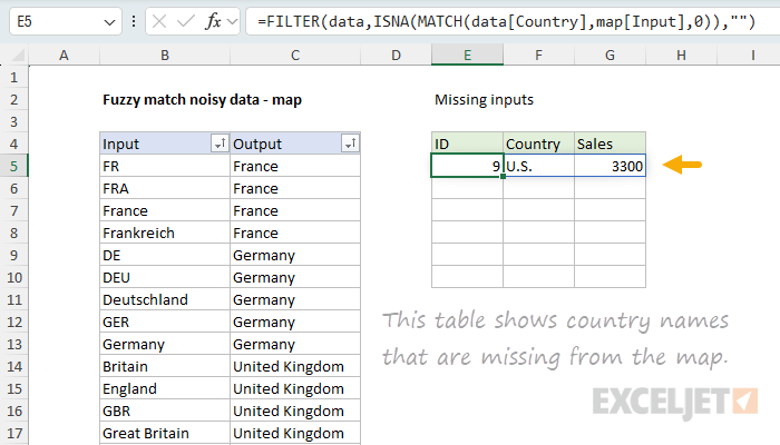
The formula in cell E5 looks like this:
=FILTER(data[],ISNA(XMATCH(data[Country],map[Input])),"")
The formula will return all unrecognized or missing country names in the source data as complete rows. Here's how it works, from the inside out:
- XMATCH function tries to find each
data[Country]value inmap[Input]. When it finds a match, it returns a position number. When it doesn't, it returns#N/A. We use XMATCH instead of MATCH here because XMATCH defaults to exact match, which saves us an argument. - ISNA function converts that result to TRUE for
#N/A(a missing input) and FALSE for everything else. - FILTER function then returns just the rows from the source table where ISNA is TRUE.
- The final argument
""tells FILTER to display an empty string when nothing matches the filter (i.e., when the map is complete).
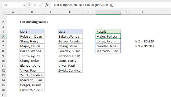
When the map is complete, the result of this formula is empty. When a new variation appears in the data, the row immediately shows up here as a clear signal that the map needs to be extended. This makes maintaining the map straightforward, since you don't have to inspect the data manually to look for new variations. For another take on this formula, see list missing values.
Try it: Add a new country name variant to the source data to see what happens.
Why a map table is a good solution
There are several reasons this approach works well:
- It's repeatable. As long as the map table is up to date, the result is the same every time. There are no thresholds, no "almost matched" values to second-guess.
- It's easy to audit. Anyone can open the map table and see exactly how each variation is being handled and which, if any, are not recognized. There is no hidden behavior.
- It's dynamic. Because the source data is in an Excel Table, the formula automatically picks up new rows. Because the map is also in an Excel Table, you can add new variations at any time, and the formula will use them on the next calculation.
- It scales. The same map can be applied to a dataset of 30 rows, 30,000 rows, or 300,000 rows. As long as the map covers the variations in the data, the formula handles the rest.
- It's a reusable pattern. Once you've built a map, you can apply the same idea to any dataset with the same problem.
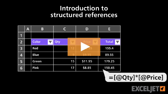
This is also a good example of how Excel Tables can be useful. You get two key benefits for free. First, Excel Tables create dynamic ranges. When a new row is added to the source data or a new variation is added to the map, every formula that references the table picks up the change automatically. No more inputting ranges like $B$5:$B$34 and updating them by hand. Second, Excel Tables give you structured references. A reference like data[Country] or map[Input] tells you exactly what you're pointing at, which makes formulas far easier to read, write, and troubleshoot. In short, Excel Tables turn a fragile, hard-to-read formula into something clear and self-maintaining.
Formula for older versions of Excel
The main formula above relies on GROUPBY, which is only available in Excel 365. If you don't have GROUPBY, you can still use the map table approach with a helper column and a regular VLOOKUP function. The trick is to do the normalization in a column on the source data, then summarize the normalized column.
Add a new column to the source data called Country (clean) with this formula:
=VLOOKUP([@Country],map,2,FALSE)
- The lookup_value is
[@Country], the country in the current row. - The table_array is the entire map table.
- The col_index_num is 2, the Output column.
- The range_lookup is FALSE, to force an exact match.
Once the helper column is in place, the easiest way to summarize the data is with a Pivot Table. Insert a Pivot Table from the source data, drag Country (clean) to the Rows area, and drag Sales to the Values area. The Pivot Table will give you the same summary as the GROUPBY formula above.
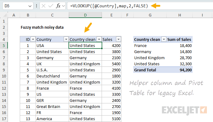
The trade-off is that a Pivot Table needs to be manually refreshed when the source data changes. The GROUPBY formula updates automatically.
Final thoughts
It's tempting to look for a clever "algorithmic" solution to a noisy data problem, but in many real cases, the most reliable solution is to build a small map table and look values up. The hardest part is creating the map, but using the UNIQUE function as a starting point makes the process a lot easier. Once the map exists, a single XLOOKUP and GROUPBY formula gives you a clean, dynamic summary, and a small FILTER-based helper makes it easy to maintain the map table as new data arrives.