Summary
To filter data with multiple criteria that are all optional, you can use the FILTER function with the LET function. In the example shown, the formula in B5 is:
=LET(
  all,SEQUENCE(ROWS(movies))^0,
  year,IF(C2="",all,movies[Year]=C2),
  director,IF(D2="",all,ISNUMBER(SEARCH(D2,movies[Director]))),
  actor,IF(E2="",all,ISNUMBER(SEARCH(E2,movies[Cast]))),
  FILTER(movies,year*director*actor,"No match")
)
where movies is an Excel Table that contains 500 movies. The inputs in C2, D2, and E2 are all optional: when an input is empty, the formula ignores that criteria and returns all records that match the criteria that remain. See below for a detailed explanation, and a variation that uses data validation to enter criteria with dropdown lists.
Generic formula
=LET(
  all,SEQUENCE(ROWS(data))^0,
  c1,IF(A1="",all,data[Col1]=A1),
  c2,IF(B1="",all,ISNUMBER(SEARCH(B1,data[Col2]))),
  FILTER(data,c1*c2,"No match")
)
Explanation
In this example, the goal is to create a simple search form to filter a list of movies with three inputs: Year, Director, and Actor. The challenge is that each input is optional, so the formula must handle any combination of inputs, including no inputs at all. This example is based on a question from a reader who wanted to find plays by a given actor, where the actor names for each play were stored as comma-separated text. To illustrate a general solution, I created a small movie database to make it easy to test the approaches explained below.
Table of contents
- The data
- The problem
- Why not Excel Table filters?
- The FILTER function
- Making criteria optional
- Searching comma-separated text
- Putting it all together
- Using data validation for inputs
- Making the formula more compact
- Blank cells in the data
- Summary
The data
The source data is stored in an Excel Table named movies that contains 500 well-known movies released since 1970. The table has four columns: Movie, Year, Director, and Cast, and the Cast column contains the main actors in each movie as comma-separated text:
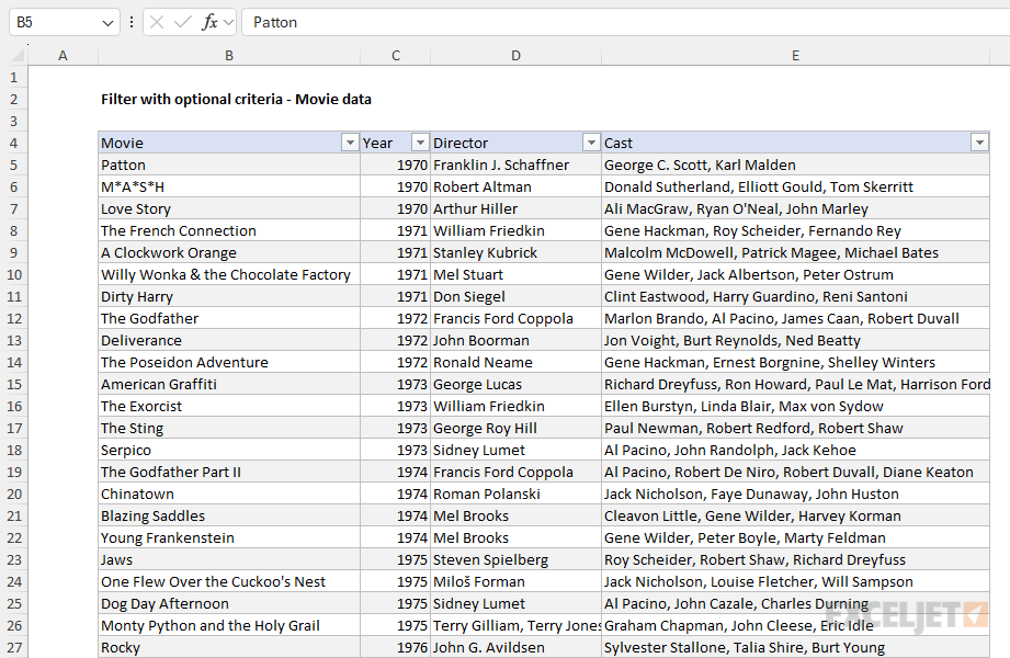
Because the data is in a table, the formula can refer to the columns with structured references like movies[Year] and movies[Cast]. As a bonus, the table will expand automatically when new movies are added, and the formula results will update to match.
The problem
The search form sits on a separate worksheet. The three inputs appear in C2 (Year), D2 (Director), and E2 (Actor), and results spill into the range below starting in cell B5. The requirements look like this:
- All three inputs are optional. An empty input should be ignored.
- The Year input should match years exactly.
- The Director and Actor inputs should support partial matching, so that "damon" will match "Matt Damon".
- The Actor input must work with the comma-separated text in the Cast column.
Why not Excel Table filters?
Since the data is already in an Excel Table, why not just use the built-in filter controls that tables provide? In many cases these controls may be all you need: they support exact match and "contains" searches, date grouping, and logical comparisons. However, there are some disadvantages. Each column must be filtered individually, the criteria are hidden when the filter menus are closed, and resetting a table back to an unfiltered state is annoying. (The fastest way I know is to toggle the filter controls off and on again with the keyboard shortcut Ctrl + Shift + L.) In addition, filtering with an Excel Table hides rows in the worksheet, which can cause problems if the worksheet displays important data to the side of the table.
By contrast, the formula approach is fast and lightweight, with some unique advantages of its own:
- Results update instantly as you enter text, and all criteria stay visible on the worksheet at a glance.
- The source data remains untouched; results land in a separate location, where they can feed other formulas.
- Match behavior can be customized per field, like the exact match on Year and the partial match on Cast above. Partial matching inside comma-separated text is where table filters start to feel clunky.
- No rows are hidden in the worksheet. You can even move the input cells used for filtering to the side of the table and they will remain visible as the data is filtered in different ways.
The solutions explained below extract matching records. Another approach not covered here is to highlight matching records in place. For a demo of this idea, see this video on building a search box with conditional formatting.
The FILTER function
The FILTER function is a natural foundation for this problem, because it is designed to extract matching records from a set of data based on a logical filter. The general structure of the formula looks like this:
=FILTER(movies,year*director*actor,"No match")
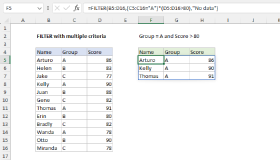
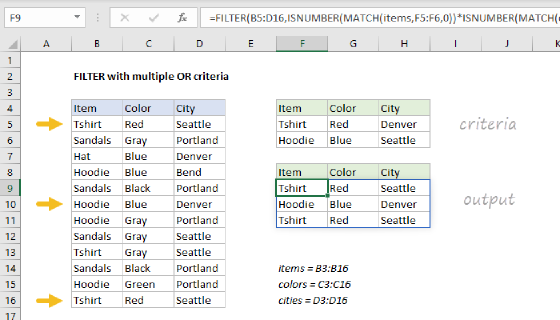
Here, year, director, and actor each represent an array of TRUE and FALSE values, one for each row in the data, created by testing one input against one column. The three arrays are multiplied together, which joins the conditions with AND logic: a row survives the filter only when all three tests return TRUE. This is a form of Boolean logic, explained in more detail in FILTER with multiple criteria. The last argument, if_empty, supplies the message "No match" when no records survive the filter.
The tricky part of this problem is making all three conditions optional. If the Year input is empty, the expression movies[Year]=C2 will return FALSE for every row, and the multiplication will zero out the whole filter. We need each test to "step aside" when its input is empty.
Making criteria optional
The main trick in this formula is to create a default array of 1s to stand in for a test when an input is empty. Since multiplying by 1 has no effect, a test that returns all 1s effectively removes itself from the filter. The array is created with the SEQUENCE function like this:
SEQUENCE(ROWS(movies))^0 // array of 1s
The ROWS function returns the number of rows in the data (500), and SEQUENCE returns the array {1;2;3;...;500}. Raising the array to the power of zero converts every number to 1, since any number raised to zero is 1. The result is an array of 500 1s, the same size as one column of the data. Note this is just a compact way to create an array of 1s; the formula below does the same thing by asking SEQUENCE for 500 numbers that start at 1 and increment by zero:
=SEQUENCE(ROWS(movies),,1,0) // also an array of 1s
With the all array defined, each condition is wrapped in an IF function that checks for an empty input:
IF(C2="",all,movies[Year]=C2)
When C2 is empty, the test returns all (match everything). When C2 contains a year, the test returns the TRUE and FALSE values from comparing the Year column to C2.
You might wonder why we go to the trouble of creating a complete array of 1s when it seems like we could just use a single TRUE like this:
IF(C2="",TRUE,movies[Year]=C2) // looks fine, but can break
The problem is the include argument of FILTER, which must be an array with one value per row in the data. When an input is empty, the version above returns a single TRUE value instead of an array. As long as at least one input contains a value, the math still works, because the single TRUE is broadcast against the other arrays during multiplication. However, when all inputs are empty, the include argument collapses to a single scalar value, and FILTER returns a #VALUE! error. In other words, the formula breaks in its default state, before a user has entered anything at all. Substituting a complete array of 1s keeps the include argument the correct size in every case.
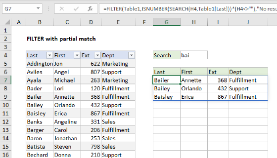
Note: this is the opposite of the problem solved in FILTER with partial match, where an empty input should return no results, and the expression (H4<>"") is used to cancel the filter when the input is empty. In this example, we want an empty input to match all results, so we substitute an array of 1s instead. The "right" answer here depends on the use case: Should the default state show all records, or should it show no records?
Searching comma-separated text
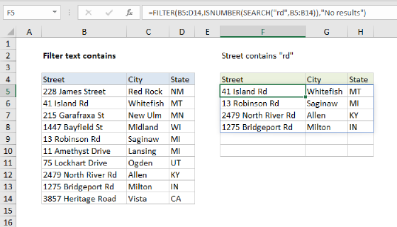
The Year test uses an exact match, but the Director and Actor tests need "contains" behavior, since a partial name like "damon" should match "Matt Damon", and the Cast column holds more than one name per cell. FILTER does not support wildcards, so we use the ISNUMBER function with the SEARCH function instead:
ISNUMBER(SEARCH(E2,movies[Cast]))
The SEARCH function looks for the text in E2 inside each cell in the Cast column. When SEARCH finds the text, it returns a number that corresponds to the position of the text:
=SEARCH("damon","Matt Damon, Robin Williams, Ben Affleck") // returns 6
When SEARCH doesn't find the text, it returns a #VALUE! error. The ISNUMBER function converts this result into TRUE or FALSE: TRUE when SEARCH returns a number (a match), and FALSE when SEARCH returns an error (no match). Because SEARCH simply looks for the text anywhere in the cell, comma-separated text works fine; a name is found no matter where it appears in the list. SEARCH is also not case-sensitive, so "damon" matches "Damon". This ISNUMBER + SEARCH pattern is a classic way to check a cell for specific text, explained in detail here.
Putting it all together
The LET function lets us name each part of the formula and assemble the logic in readable steps:
=LET(
  all,SEQUENCE(ROWS(movies))^0,
  year,IF(C2="",all,movies[Year]=C2),
  director,IF(D2="",all,ISNUMBER(SEARCH(D2,movies[Director]))),
  actor,IF(E2="",all,ISNUMBER(SEARCH(E2,movies[Cast]))),
  FILTER(movies,year*director*actor,"No match")
)
Working through the names one at a time:
allis an array of 500 1s, used as the default "match everything" test.yearreturnsallwhen C2 is empty. Otherwise, it compares the Year column to C2 with an exact match.directorreturnsallwhen D2 is empty. Otherwise, it performs a partial match of D2 against the Director column with ISNUMBER + SEARCH.actorreturnsallwhen E2 is empty. Otherwise, it performs a partial match of E2 against the Cast column with ISNUMBER + SEARCH.- Finally, FILTER multiplies the three arrays together and returns the matching records, or "No match" when nothing survives the filter.
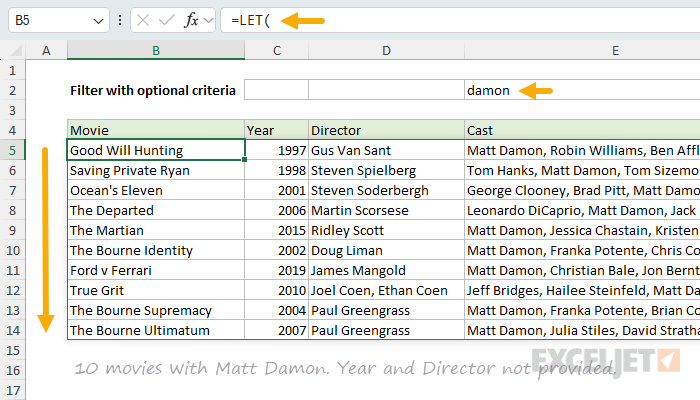
In the worksheet below, "damon" has been entered in E2 with no Year or Director. The formula returns the 10 movies in the data that include Matt Damon in the Cast column:
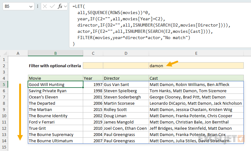
Since the year and director tests both return an array of 1s, the actor test alone determines the result. If a year like 2010 is added in C2, the results narrow further, and clearing all three inputs returns all 500 movies.
Tip: to display a result message like "10 of 500 movies" on the worksheet, you can use a formula like this:
=ROWS(B5#)&" of "&ROWS(movies)&" movies". The B5# reference is the spill range returned by the formula in B5.
Using data validation for inputs
Typing partial names works well when you know the data, but you can also use data validation to select a director or actor from a dropdown list. In this variation, the formula is the same except for the director test, which becomes an exact match, since a value selected from a list is always complete:
=LET(
  all,SEQUENCE(ROWS(movies))^0,
  year,IF(C2="",all,movies[Year]=C2),
  director,IF(D2="",all,movies[Director]=D2),
  actor,IF(E2="",all,ISNUMBER(SEARCH(E2,movies[Cast]))),
  FILTER(movies,year*director*actor,"No match")
)
Note the actor test still uses ISNUMBER + SEARCH, because the Cast column contains more than one name per cell, so an exact match against the full cell would fail.
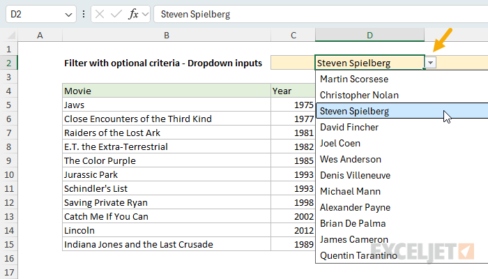
In the worksheet below, "Steven Spielberg" has been selected from the dropdown list in D2, and the results update instantly:
To provide values for the dropdown lists, we need a unique list of directors and a unique list of actors, created on a separate helper sheet. For directors, one simple option is the UNIQUE function with the SORT function:
=SORT(UNIQUE(movies[Director]))
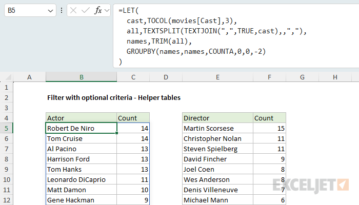
In this case, I've opted to use the GROUPBY function instead, which makes it easy to generate a count of movies for each director at the same time. The formula in E5 on the helper sheet is:
=GROUPBY(movies[Director],movies[Director],COUNTA,0,0,-2)
GROUPBY groups the Director column by unique value, counts the movies for each director with COUNTA, and sorts the results in descending order by count. Note that GROUPBY is only available in Excel 365.
The actor list is a harder problem, because the names must first be extracted from the comma-separated text in the Cast column. The formula in B5 on the helper sheet handles this with the TOCOL, TEXTJOIN, and TEXTSPLIT functions:
=LET(
  cast,TOCOL(movies[Cast],3),
  all,TEXTSPLIT(TEXTJOIN(",",TRUE,cast),,","),
  names,TRIM(all),
  GROUPBY(names,names,COUNTA,0,0,-2)
)
Working from the inside out: TOCOL collects the Cast column into a single array that spills all values in one column, TEXTJOIN joins all of the text into one comma-separated string, and TEXTSPLIT splits the string back into one name per row. The TRIM function removes the stray spaces left over after the commas, and GROUPBY again returns unique names with a count, sorted in descending order.
The structure of the formula above, which involves joining all text into one string before processing with TEXTSPLIT, is a workaround for Excel's array of arrays limitation. It works fine in this case, but be aware that it will fail on a larger set of data. The limit hits inside TEXTJOIN, which can return a maximum of 32,767 characters (the most a single cell can hold), and all of the cast names must fit into this one string. To avoid the limit entirely, you can process the data row by row with REDUCE and VSTACK, as explained in this example.
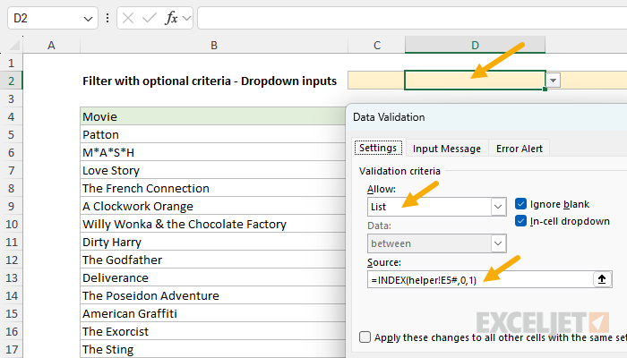
Because GROUPBY returns both names and counts, the last step is to extract just the first column for each dropdown. The data validation rule for Director (D2) uses the INDEX function like this:
=INDEX(helper!E5#,0,1)
The screen below shows the completed data validation rule for D2:
And the rule for Actor (E2) looks like this:
=INDEX(helper!B5#,0,1)
INDEX is the traditional way to slice one column out of an array; the newer CHOOSECOLS function would work just as well.
Making the formula more compact
Excel formula experts love to tinker with formulas to make them shorter. After this page was published, reader and Excel formula wiz Matt Hanchett wrote in with a more compact version of the formula. As a reminder, the original formula looks like this:
=LET(
  all,SEQUENCE(ROWS(movies))^0,
  year,IF(C2="",all,movies[Year]=C2),
  director,IF(D2="",all,ISNUMBER(SEARCH(D2,movies[Director]))),
  actor,IF(E2="",all,ISNUMBER(SEARCH(E2,movies[Cast]))),
  FILTER(movies,year*director*actor,"No match")
)
Here is Matt's version:
=LET(
  year,(C2="")+(movies[Year]=C2),
  director,ISNUMBER(SEARCH(D2,movies[Director])),
  actor,ISNUMBER(SEARCH(E2,movies[Cast])),
  FILTER(movies,year*director*actor,"No match")
)
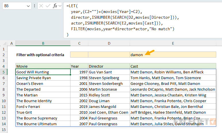
The results are exactly the same. In the worksheet below, "damon" has been entered as the actor and Matt's formula in B5 returns the same 10 matching movies:
Notice that the all variable and the three IF functions are gone. Let's take a look at how this works. First, note that the last line of the formula is unchanged, and still determines the final result:
FILTER(movies,year*director*actor,"No match")
The key thing to understand is that by the time we reach this line, year, director, and actor are all arrays that contain 500 values, one for each movie in the table. When the three arrays are multiplied together, the result is a single array of numbers. Any row with a non-zero result makes it through FILTER, and any row with a zero gets blocked.
The main idea used to shorten the formula appears in the year variable:
(C2="")+(movies[Year]=C2)
The expression (C2="") returns a single TRUE or FALSE value. The expression (movies[Year]=C2) compares each year in the table to the value in C2 and returns an array of 500 TRUE and FALSE values. When these two results are added together, Excel coerces TRUE to 1 and FALSE to 0, and the result is a single array of 500 numbers.
Now consider what happens in each case. When C2 is empty, (C2="") returns TRUE, which behaves like 1. And since every movie has a year, comparing the Year column to an empty cell returns 500 FALSE values. Adding 1 to this array creates an array of 500 1s, which causes FILTER to ignore the year test altogether. When C2 contains a year, (C2="") returns FALSE, which behaves like 0, so the addition has no effect. The result is an array of 1s and 0s, where the 1s represent movies with a year that matches C2. In other words, adding (C2="") does the same job as the IF function in the original formula, in less space.
Another way to read the addition is as OR logic: a movie passes the year test when C2 is blank, or when the year in C2 matches the movie's year. This is standard Boolean algebra, where addition works like OR, and multiplication works like AND. You can see the same idea at work in the last line of the formula, where multiplication joins the three tests with AND logic. For a quick overview of how this works in Excel, see this video on Boolean algebra.
We could use exactly the same trick to remove the IF functions for director and actor like this:
=LET(
  year,(C2="")+(movies[Year]=C2),
  director,(D2="")+ISNUMBER(SEARCH(D2,movies[Director])),
  actor,(E2="")+ISNUMBER(SEARCH(E2,movies[Cast])),
  FILTER(movies,year*director*actor,"No match")
)
But Matt's version doesn't do this for director and actor. Why not? It turns out that the SEARCH function has a useful edge case: when find_text is empty (""), SEARCH returns 1 instead of an error, because an empty string is found at the start of any text. That means that when D2 is empty, ISNUMBER(SEARCH(D2,movies[Director])) already returns TRUE for every row in the table, so we get the "match everything" behavior for free, and (D2="")+ isn't needed at all:
=LET(
  year,(C2="")+(movies[Year]=C2),
  director,ISNUMBER(SEARCH(D2,movies[Director])),
  actor,ISNUMBER(SEARCH(E2,movies[Cast])),
  FILTER(movies,year*director*actor,"No match")
)
This behavior can be surprising, but it is by design and works reliably (as long as the searched column has no empty cells, see below), and it's a handy thing to know when you are building a formula that performs a text search. See Empty search string for details. The REGEXTEST function behaves the same way with an empty pattern, so it can stand in for SEARCH here when you need case-sensitive or regex-based matching.
Finally, we could take things one step further and remove the LET function altogether:
=FILTER(
  movies,
  ((C2="")+(movies[Year]=C2))*
  ISNUMBER(SEARCH(D2,movies[Director]))*
  ISNUMBER(SEARCH(E2,movies[Cast])),
  "No match"
)
Note the extra parentheses around the year test. Because Excel performs multiplication before addition, the parentheses are needed to make sure (C2="") is added to the year test only, and not to the result of the entire multiplication. Without them, the formula contains a subtle bug: whenever C2 is blank, every movie passes the filter, no matter what director or actor has been entered. A good reminder that the devil is always in the details with advanced Excel formulas.
So which version should you use? This really comes down to personal preference. Years ago, before dynamic array formulas arrived, I used to work harder to make formulas shorter, with the idea that any formula that didn't fit on one line was automatically a "complex formula". These days, I don't worry about it as much. Many useful formulas are more than one line by design, and the most important thing is readability. One exception: if your data has empty cells, read the next section before you pick the compact version.
Blank cells in the data
The movie data has no empty cells, but real data often does. After this page was published, a reader applied the formula to an orders table where some columns can legitimately be blank, and ran into two problems.
First, the compact formula above can drop records. It relies on SEARCH returning 1 when the search text is empty, but SEARCH returns #VALUE! when the cell being searched is empty, even if the search text is also empty. So when D2 is empty, a movie with no director fails the director test and quietly disappears from the results. The fix is to add the empty-input test back to the text tests, the same way it works for year:
=LET(
  year,(C2="")+(movies[Year]=C2),
  director,(D2="")+ISNUMBER(SEARCH(D2,movies[Director])),
  actor,(E2="")+ISNUMBER(SEARCH(E2,movies[Cast])),
  FILTER(movies,year*director*actor,"No match")
)
The original formula at the top of the page does not have this problem, because IF returns the array of 1s before SEARCH ever runs.
Second, FILTER displays empty cells in the results as zeros, which is a general quirk of FILTER. To show them as blank instead, replace empty cells with empty strings ("") before filtering:
FILTER(IF(movies="","",movies),year*director*actor,"No match")
Numbers and dates are not affected; only the empty cells change.
Summary
To filter data with optional criteria in Excel:
- Use the FILTER function with one logical test per input, and multiply the tests together to apply AND logic.
- Create a default array of 1s with
SEQUENCE(ROWS(data))^0, and use IF to substitute the default when an input is empty, so empty inputs match all records. - Use ISNUMBER + SEARCH for "contains" matching; it handles partial names and comma-separated text.
- Use LET to name each test and keep the formula readable.
- To drive inputs with dropdown lists, build unique value lists with GROUPBY (or UNIQUE and SORT) and switch the corresponding test to an exact match.
- For a more compact formula, Boolean addition (OR logic) can replace the IF functions, as explained above.
- If the data has empty cells, keep the empty-input test on SEARCH-based criteria, and use
IF(data="","",data)inside FILTER to show empty cells as blanks instead of zeros.
The FILTER, LET, and SEQUENCE functions are all available in Excel 2021+ and Excel 365. The helper formulas above also use TOCOL and TEXTSPLIT (available in Excel 2024+ and Excel 365) and GROUPBY (Excel 365 only).