Drag formula down step column reference

Summary

To copy a formula down a column while its references move across columns, you can use the OFFSET function with a counter based on the ROWS function. In the example shown, the formula in C13 is:

=SUM(OFFSET($C$5,0,ROWS(C$13:C13)-1),OFFSET($C$7,0,ROWS(C$13:C13)-1))

As the formula is copied down, the references step across from column C to D, E, and F, and the formula returns the total for products A and C in each quarter. See below for an alternative based on the INDEX function, and a single formula option based on the TRANSPOSE function.

Generic formula

=OFFSET(first,0,n)

Where first is an absolute reference to the first cell, and n is a counter that returns 0, 1, 2, etc. as the formula is copied down.

Explanation

In this example, the goal is to total sales for products A and C in each quarter. The data has one row per product, and the quarters run across in columns C, D, E, and F. The summary in B12:C16 lists the quarters going down. This means the formula in C13 needs to be dragged down vertically while its references step across horizontally, which is something a normal formula won't do.

This is a surprisingly common problem, and it can be hard to describe. You might think of it as "drag a formula down but change the column reference", or "fill down, move across", etc.

The problem
A counter with ROWS
OFFSET solution
INDEX alternative
TRANSPOSE option
All products
Drag across, step down
Summary

The problem

If you enter formulas manually, this problem is simple. These are the formulas we need in C13:C16:

=SUM(C5,C7) // Q1
=SUM(D5,D7) // Q2
=SUM(E5,E7) // Q3
=SUM(F5,F7) // Q4

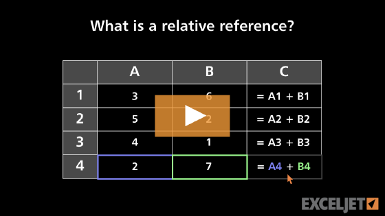
Notice the rows stay the same, and the column changes at each new row: C, D, E, F. The challenge is how to create a formula that will step references across columns as it is copied down. A relative reference changes only in the direction the formula is copied. When a formula is copied down, the row numbers change and the column letters do not. If you copy =SUM(C5,C7) down one row, you get =SUM(C6,C8), not =SUM(D5,D7). Locking the rows with a mixed reference like C$5 doesn't help, because the column still won't change.

One solution is to abandon the idea of the references changing by themselves and instead, lock each reference to a starting point, and use a counter that will work as an offset when the formula is copied down. Let's look first at how to construct a counter.

A counter with ROWS

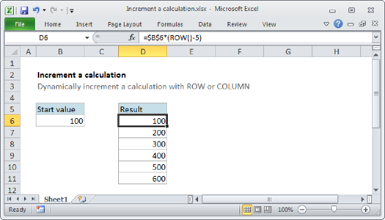
A nice way to create a counter is to use the ROWS function with an expanding reference:

=ROWS(C$13:C13)

ROWS returns the number of rows in a range. Because the first reference is locked to row 13 and the second reference is relative, the range expands as the formula is copied down, and ROWS returns a larger number at each new row:

=ROWS(C$13:C13) // returns 1
=ROWS(C$13:C14) // returns 2
=ROWS(C$13:C15) // returns 3
=ROWS(C$13:C16) // returns 4

You will sometimes see a formula use a counter like =ROW()-12 for the same purpose. While this works (and is somewhat easier to read) the hardcoded 12 depends on where the formula sits in the worksheet. If a row is inserted above the summary, the counter will return the wrong numbers. The expanding reference solves this problem.

In the formulas below, n stands for this counter.

OFFSET solution

The OFFSET function is designed for exactly this kind of problem. OFFSET returns a reference that is a given number of rows and columns away from a starting point. To start at C5 and move n columns to the right, the generic formula looks like this:

=OFFSET($C$5,0,n)

The starting cell is an absolute reference, so it won't change when the formula is copied. The rows argument is zero, since we want to stay in the same row. The cols argument is n. For OFFSET, we want n to begin at zero, so that the first formula returns C5 itself. To make that happen, we subtract 1 from the counter explained above:

=OFFSET($C$5,0,ROWS(C$13:C13)-1)

Now we have what we need to build the final formula. The basic idea is to replace each reference that needs to change with OFFSET, and leave the rest of the formula alone. The manual formula =SUM(C5,C7) has two references, so the formula in C13 uses OFFSET twice:

=SUM(OFFSET($C$5,0,ROWS(C$13:C13)-1),OFFSET($C$7,0,ROWS(C$13:C13)-1))

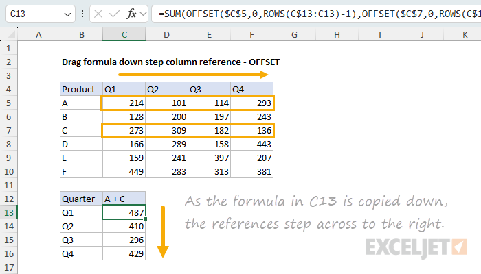
Drag formula down and step column reference with OFFSET

As the formula is copied down, the counter increases by one at each row, and OFFSET returns references like this:

=SUM(C5,C7) // C13, n=0
=SUM(D5,D7) // C14, n=1
=SUM(E5,E7) // C15, n=2
=SUM(F5,F7) // C16, n=3

These are the same formulas we entered manually above.

Note: OFFSET is a volatile function, which means it recalculates with every worksheet change. In a small worksheet, you won't notice any difference. In a large or complicated workbook, OFFSET formulas can make Excel feel slow. If you run into this problem, switch to the INDEX alternative below.

INDEX alternative

The INDEX function returns the value at a given position in a range. To solve this problem with INDEX, we give INDEX the full row as an absolute reference and use the counter to ask for the nth value:

=INDEX($C$5:$F$5,n)

INDEX counts from 1, so we can use the counter as-is. The recipe is the same as before: wrap each reference that needs to step across. The formula in C13 is:

=SUM(INDEX($C$5:$F$5,ROWS(C$13:C13)),INDEX($C$7:$F$7,ROWS(C$13:C13)))

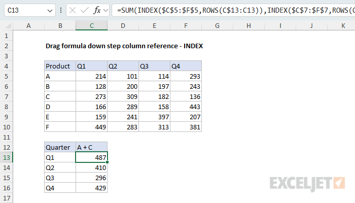
Drag formula down and step column reference with INDEX

As the formula is copied down, the first INDEX returns the 1st, 2nd, 3rd, and 4th values in row 5, and the second INDEX returns the same values from row 7. The results are the same as the OFFSET formula above. The difference is that INDEX is not volatile, so this version is a better choice in a large or complicated workbook. The tradeoff is that INDEX needs the full range (C5:F5), where OFFSET needs only the first cell.

Another way to set up INDEX is to lock the entire block of data, and provide both a row number and a column number:

=SUM(INDEX($C$5:$F$10,1,n),INDEX($C$5:$F$10,3,n))

Here, the row number is hardcoded as 1 for product A and 3 for product C, and n selects the quarter.

TRANSPOSE option

The formulas above follow the way most people think about this problem: a confounding problem with Excel references. However, in Excel 2021+ and Excel 365, dynamic array formulas enable a different approach: don't copy the formula at all. Instead, calculate all four totals at once, and use the TRANSPOSE function to flip the result from horizontal to vertical. The formula in C13 is:

=TRANSPOSE(C5:F5+C7:F7)

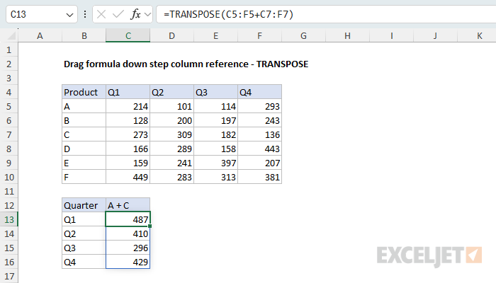
One TRANSPOSE formula in place of a formula copied down

Inside TRANSPOSE, the two ranges are added together. Because each range contains four values, the result is a horizontal array with four totals:

=TRANSPOSE({487,410,296,429})

TRANSPOSE then converts the horizontal array into a vertical array, and the four results spill into the range C13:C16. There is no counter, and nothing to copy. This is the simplest solution when it fits the problem. Note that a formula like this won't work inside an Excel Table, and you can't override one result without replacing the entire formula. In those cases, use OFFSET or INDEX.

All products

In the example above, the formula sums two specific products. A simpler version of the same problem is to sum all products in each quarter. Entered manually, the formulas are =SUM(C5:C10), =SUM(D5:D10), and so on. In this case, only one reference needs to step across, but it is a range and not a single cell. With OFFSET, provide a height and width to return a range that is 6 rows by 1 column:

=SUM(OFFSET($C$5,0,ROWS(C$13:C13)-1,6,1))

With INDEX, provide zero for the row number, which causes INDEX to return the entire column:

=SUM(INDEX($C$5:$F$10,0,ROWS(C$13:C13)))

In Excel 2024+ and Excel 365, the BYCOL function can sum each column in one step, and TRANSPOSE will flip the result:

=TRANSPOSE(BYCOL(C5:F10,SUM))

Drag across, step down

The same problem occurs in the other direction: a formula is dragged horizontally, and the references need to step vertically. The solution is the same, with two changes. The counter is based on the COLUMNS function, and the counter goes into the rows argument of OFFSET. In the worksheet below, the goal is to total Q1 and Q3 for each product, with the products listed across. The formula in C13, copied across, is:

=SUM(OFFSET($C$5,COLUMNS($C13:C13)-1,0),OFFSET($E$5,COLUMNS($C13:C13)-1,0))

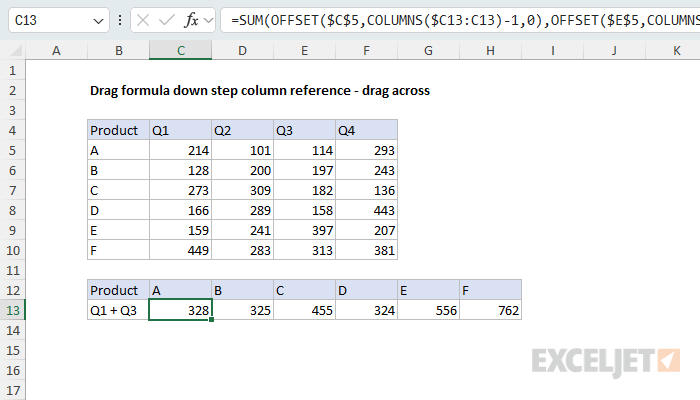
Drag formula across and step row reference

As the formula is copied to the right, COLUMNS returns 1, 2, 3, etc. and OFFSET moves down one row at each new column. The INDEX version works the same way, with a vertical range like INDEX($C$5:$C$10,n).

Summary

Relative references change only in the direction a formula is copied. A formula copied down will never change columns by itself.
To step a reference across while copying down, lock the reference and move it with a counter like ROWS(C$13:C13).
OFFSET is the most direct solution: OFFSET(first,0,n) with a counter that starts at zero. OFFSET is volatile, and can slow down a large workbook.
INDEX is the non-volatile alternative: INDEX(range,n) with a counter that starts at 1.
In Excel 2021+ and Excel 365, a single TRANSPOSE formula can often replace the copied formulas altogether.
To drag a formula across and step down, use COLUMNS for the counter.