Data validation allow letters and numbers only

Summary

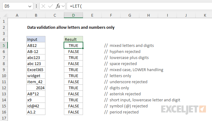
To create a data validation rule that allows only letters and numbers (no punctuation, symbols, or spaces), you can use a custom formula based on the FIND, SEQUENCE, and LET functions. In the example shown, the data validation applied to B5:B16 is:

=LET(
input,B5,
allowed,"abcdefghijklmnopqrstuvwxyz0123456789",
chars,MID(LOWER(input),SEQUENCE(LEN(input)),1),
result,AND(ISNUMBER(FIND(chars,allowed))),
result
)

The formula splits the value entered in B5 into individual characters, then checks each character against the characters in allowed. The formula returns TRUE only when every character passes, otherwise it returns FALSE. Values that contain any character outside the allowed list are rejected. To make the logic easier to understand and test, the formula is entered in column D, where it displays the TRUE or FALSE result for each input in column B. See below for a detailed explanation, a simpler option based on the REGEXTEST function (Excel 365), and an option that works in older versions of Excel.

Note: This formula uses the LET and SEQUENCE functions, available in Excel 2021+ and Excel 365. For earlier versions of Excel, see the SUMPRODUCT option below.

Generic formula

=LET(
input,A1,
allowed,"abcdefghijklmnopqrstuvwxyz0123456789",
chars,MID(LOWER(input),SEQUENCE(LEN(input)),1),
result,AND(ISNUMBER(FIND(chars,allowed))),
result
)

Explanation

In this example, the goal is to create a data validation rule that only accepts letters (a-z) and numbers (0-9). This is a common requirement for values like product codes, usernames, and IDs, where spaces, punctuation, and symbols will cause problems in other systems. Excel has no built-in rule for this kind of check, so we need a custom formula. The basic approach is to split the input value into individual characters, then check that every character exists in a list of allowed characters. The sections below explain each step in detail.

Table of contents

• How data validation formulas work
• Splitting text into characters
• Testing each character
• Why FIND instead of SEARCH
• Customizing the allowed characters
• The formula without LET
• A simpler option: REGEXTEST
• Older versions of Excel
• Summary

How data validation formulas work

Data validation rules are triggered when a user adds or changes a cell value. When a rule is based on a custom formula, the formula must return TRUE for the input to be accepted. If the formula returns FALSE, the input is rejected, and Excel displays an error window. To apply the rule, select the input range, then enter the formula in the Data Validation dialog (Data > Data Validation > Allow > Custom):

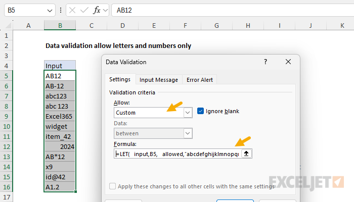
Cell references in data validation formulas are relative to the upper left cell in the range selected when the validation rule is defined. In this case, the rule is applied to B5:B16, so the formula refers to B5, and Excel adjusts the reference for each cell in the range automatically.

One challenge with custom validation formulas is that the formula box in the dialog is small, and Excel gives you no feedback about what the formula is doing. It also doesn't display line breaks, which takes the fun out of using LET. A good process is to develop the formula on the worksheet first, next to sample input, where you can see the TRUE or FALSE result directly. That is the purpose of the formulas in column D in the worksheet above: they run the same logic as the validation rule, one row at a time. Once the formula behaves correctly, port it into the Data Validation dialog.

Note: By default, the "Ignore blank" setting is enabled, so clearing a cell will not trigger validation. For an overview of how data validation works, including how to enter and manage rules, see our complete guide to data validation.

Splitting text into characters

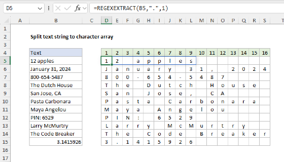
The first job of the formula is to break the entered value into individual characters. Excel does not have a dedicated function for splitting a text string into an array of characters, so we use a common pattern based on the MID and SEQUENCE functions when the chars variable is defined:

chars,MID(LOWER(input),SEQUENCE(LEN(input)),1)

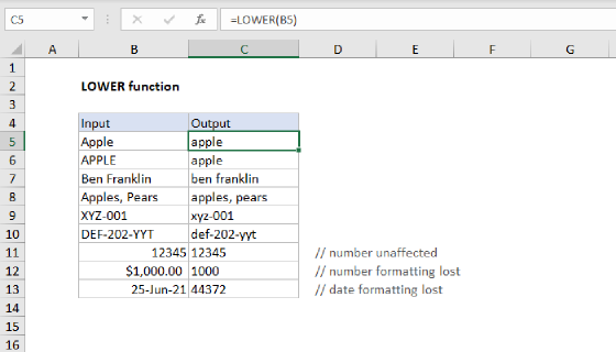
Working from the inside out, the LOWER function first converts the input to lowercase. This is how the formula handles capital letters: rather than listing both "a" and "A" as allowed characters, we convert everything to lowercase before checking. Next, the LEN function returns the number of characters in the input, and the SEQUENCE function uses that count to generate a list of numbers, one for each character position. For example, if a user enters "AB12", LEN returns 4, and SEQUENCE returns an array like this:

{1;2;3;4}

These numbers are handed to the MID function as the starting position, with the length set to 1. Because MID receives four starting positions, it returns four results, one character per position:

{"a";"b";"1";"2"} // "AB12" after LOWER and MID

The result is an array that contains each character of the original input, assigned to the variable chars.

Testing each character

Now that we have the input split into characters, we need to check that each character is allowed. This is the job of the FIND function in the definition of result:

result,AND(ISNUMBER(FIND(chars,allowed)))

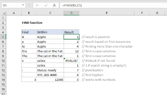
FIND locates one text string inside another and returns its numeric position. If the text is not found, FIND returns a #VALUE! error. In this formula, FIND looks for each character in chars inside the allowed string. Because chars contains multiple values, FIND returns multiple results. For the input "AB12", we get an array of four positions:

{1;2;28;29} // all characters found

All four characters exist in allowed, so all four results are numbers. Now consider what happens if a user enters "AB-12". The hyphen is not in the allowed string, so FIND returns a #VALUE! error in the third position:

{1;2;#VALUE!;28;29} // "-" not found

The ISNUMBER function converts these results into TRUE and FALSE values, where TRUE means a character was found, and FALSE means it wasn't:

{TRUE;TRUE;FALSE;TRUE;TRUE}

Finally, the AND function collapses the array into a single result. AND only returns TRUE when all values are TRUE, so a single disallowed character anywhere in the input is enough to make the formula return FALSE, which triggers the data validation rule to reject the input.

The last line of the LET formula simply returns result. This looks redundant, but it is a handy convention: to troubleshoot the formula in a worksheet, you can temporarily change the last line to chars (or any other variable) to inspect an intermediate step directly.

AND aggregate values to a single result. That can cause trouble when the goal is to return multiple values, but in this case, it's exactly what we want.

Why FIND instead of SEARCH

Excel has two functions that locate one text string inside another: FIND and SEARCH. At first glance, the SEARCH function looks like the better choice, because SEARCH is not case-sensitive, and we could skip the LOWER function altogether. However, SEARCH has a serious drawback in this formula: it supports wildcards. The characters *, ?, and ~ have special meanings to SEARCH, so an input like "AB*12" would pass validation, because SEARCH treats the asterisk as "match anything" instead of a literal character. FIND does not support wildcards and always performs a literal match, which is exactly what we want when validating input. The trade-off is that FIND is case-sensitive, and we handle that by converting the input to lowercase with LOWER before testing.

Customizing the allowed characters

One nice feature of this formula is that the validation "policy" lives in one place: the allowed variable. To change what characters are accepted, just edit the string. For example, to also allow spaces, hyphens, and underscores, append them to the end:

allowed,"abcdefghijklmnopqrstuvwxyz0123456789 -_"

Because FIND performs a literal match, you can safely add characters like *, ?, and ~ as well. To enforce a specific case (for example, uppercase letters only), remove the LOWER function and list only uppercase letters in allowed:

=LET(
input,B5,
allowed,"ABCDEFGHIJKLMNOPQRSTUVWXYZ0123456789",
chars,MID(input,SEQUENCE(LEN(input)),1),
result,AND(ISNUMBER(FIND(chars,allowed))),
result
)

With this version, an input like "ab12" will fail validation, because lowercase letters are no longer in the allowed list. See also: Data validation allow uppercase only.

Tip: To let users maintain the list of allowed characters directly on the worksheet instead of inside the formula, see Data validation specific characters only, which uses a named range to hold allowed characters.

The formula without LET

The LET function is not actually required to solve this problem. The same logic can be written as a single expression:

=AND(ISNUMBER(FIND(MID(LOWER(B5),SEQUENCE(LEN(B5)),1),"abcdefghijklmnopqrstuvwxyz0123456789")))

This formula works fine, and it is more compact. However, the compact version must be read from the inside out, starting with LOWER and working outward through five levels of nesting. The reason to use LET is readability. The LET version reads from top to bottom like a series of steps: here is the input, here are the allowed characters, split the input into characters, check each one.

Naming things also makes the formula easier to maintain. In the compact version, the allowed characters are buried in the middle of the formula, and the input cell (B5) appears twice. To change the allowed characters, or to point the rule at a different cell, you need to hunt through the nesting, and it is easy to update one reference but miss the other. In the LET version, both settings sit at the top of the formula, defined exactly once: input and allowed are the two things you might want to edit, and you can ignore the details below.

Finally, the LET version is easier to debug. Because the formula ends by returning the result variable, you can temporarily change the last line to chars or any other variable to inspect that step directly on the worksheet, as explained above. With the compact version, checking an intermediate step means breaking the formula apart by hand.

Using LET does not change what the formula does, and the performance difference here is negligible. But a well-written LET formula is self-documenting, which has value to the future user needs to understand how it works. For more about LET, including how to convert an existing formula, see the LET function page and this detailed LET example.

A simpler option: REGEXTEST

If you are using Excel 365, you can solve this problem with a much simpler formula based on the REGEXTEST function:

=REGEXTEST(B5,"^[a-zA-Z0-9]+$")

REGEXTEST checks a text value against a regular expression, a pattern that describes the structure of the text, and returns TRUE or FALSE. In this case, the pattern works like this: the caret (^) anchors the match to the start of the text, the character class [a-zA-Z0-9] matches any letter or number, the plus sign (+) requires one or more of those characters, and the dollar sign ($) anchors the match to the end of the text. Together, the pattern returns TRUE only when the entire entry consists of letters and numbers. Notice there is no need for LOWER, because the character class includes both uppercase and lowercase letters directly.

To customize the allowed characters, adjust the character class. For example, to also allow spaces, underscores, and hyphens:

=REGEXTEST(B5,"^[a-zA-Z0-9 _-]+$")

Note: REGEXTEST is available in Excel 365 only. If your workbook needs to run in Excel 2021+, use the LET formula above instead.

Older versions of Excel

In versions of Excel before 2021, LET and SEQUENCE are not available, so we need a different way to split the input into characters and aggregate the results. The formula below performs the same test with the SUMPRODUCT function:

=SUMPRODUCT(--ISNUMBER(FIND(MID(LOWER(B5),ROW(INDIRECT("1:"&LEN(B5))),1),"abcdefghijklmnopqrstuvwxyz0123456789")))=LEN(B5)

The logic is the same, but the approach is old school. The snippet based on MID, ROW, and INDIRECT splits the input into an array of characters, as explained here. FIND and ISNUMBER then test each character as before, producing an array of TRUE and FALSE values. The double negative (--) converts these values to 1s and 0s, and SUMPRODUCT adds them up to get a count of valid characters. Finally, this count is compared to the length of the input. When every character is allowed, the counts are equal and the formula returns TRUE. This version works in all versions of Excel.

Summary

To allow only letters and numbers with data validation, the formula splits input into characters, then verifies each character appears in a list of allowed characters:

• MID, SEQUENCE, and LEN split the input into an array of individual characters
• LOWER converts input to lowercase, so capital letters pass without listing them separately
• FIND checks each character against the allowed string; ISNUMBER and AND require all characters to pass
• FIND is used instead of SEARCH because SEARCH supports wildcards, which would let *, ?, and ~ slip through
• To change the validation policy, edit the allowed string in one place
• In Excel 365, the REGEXTEST function offers a simpler one-line alternative
• LET improves readability and provides documentation

For a version of this problem where allowed characters are maintained on the worksheet, see Data validation specific characters only.