Summary
Arrays are now a core part of how Excel formulas work. This article explains what arrays are, how array formulas work, and how dynamic arrays have changed the game. Includes practical examples, tips for inspecting arrays, a guide to the new array functions in Excel, and the workbook.
If you use Excel formulas on a regular basis, you need to understand arrays. Arrays used to be an advanced topic, something only power users worried about. But with the introduction of dynamic arrays, arrays are now a central part of how Excel formulas work. In this article, I'll explain what arrays are, how array formulas work, and why dynamic arrays are such a big deal. I'll also walk through practical examples and share tips for inspecting arrays when things get complicated.
Table of Contents
- Why arrays matter now
- What is an array?
- What is an array formula?
- What are dynamic arrays?
- Simple array formula examples
- Advanced array formula examples
- Arrays and ranges not always interchangeable
- How to inspect arrays in Excel
- New functions for working with arrays
- Summary
Why arrays matter now
For years, arrays lived in a nerdy world of advanced Excel formulas. Most users never thought about them, and the power users who did had to deal with the awkward syntax requirement Control + Shift + Enter (CSE). Over the past 5 years, this has completely changed.
With the introduction of dynamic arrays in Excel 365, formulas that return multiple values now spill results directly onto the worksheet. This is a fundamental change to how Excel's formula engine works, and it makes array formulas far more intuitive and useful:
- Formulas can now return multiple results that automatically spill into neighboring cells
- There is no need to enter formulas with Control + Shift + Enter
- Excel has introduced more than 25 new functions specifically designed to work with arrays
The bottom line is that arrays are no longer a geeky topic for power users. If you write formulas often, you're going to encounter arrays regularly, and understanding how they work will make you a much more effective Excel user.
Video: What are Dynamic Array formulas?
What is an array?
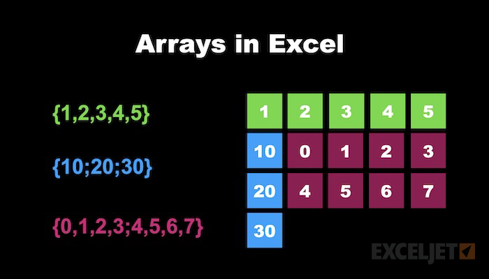
An array is simply a collection of values arranged in a specific order. If you've worked with a range of cells in Excel, you already have an intuitive understanding of arrays. In Excel formulas, arrays appear inside curly braces. A horizontal array uses commas to separate values:
{1,2,3} // horizontal array
A vertical array uses semicolons:
{1;2;3} // vertical array
And, a two-dimensional array uses both:
{1,2,3;4,5,6} // 2D array (2 rows, 3 columns)
Try it!
Note that you can enter arrays directly in the formula bar, and Excel will know what to do. To understand how this works, enter the following "formulas" into a cell on a worksheet:
={1,2,3}
={1;2;3}
={1,2,3;4,5,6}
={1,2,3}+1
={1;2;3}^2
As you might guess, arrays map perfectly to ranges. A single column of cells is a vertical array, a single row is a horizontal array, and a block of cells is a two-dimensional array. You can see how this works in the worksheet below. A range like B5:B10 is just a vertical array of 6 values.
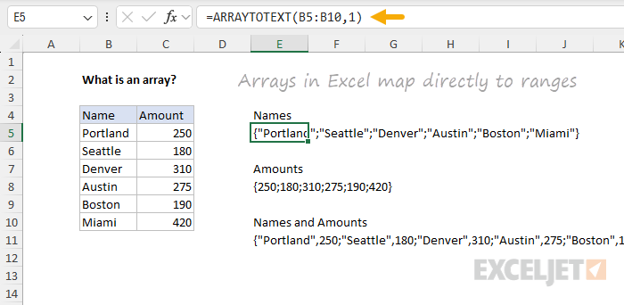
To see the array values associated with a range, we are using the ARRAYTOTEXT function. This function converts a range to a text string that shows the array. For example, the Names column (B5:B10) maps to this vertical array:
=ARRAYTOTEXT(B5:B10,1) // {"Portland";"Seattle";"Denver";"Austin";"Boston";"Miami"}
The Amounts column (C5:C10) maps to a numeric array: {250;180;310;275;190;420}. And both columns together (B5:C10) produce a two-dimensional array with commas separating columns and semicolons separating rows.
The ARRAYTOTEXT function is just one way to see the arrays behind your formulas. For more techniques, see How to inspect arrays in Excel below.
What is an array formula?
An array formula is any formula that works with an array of values rather than a single value. Many array formulas are not complicated at all. The concept is simpler than it sounds.
Here's a classic example. Say we want to find the maximum temperature change over seven days, where high temps are in C5:C11 and low temps are in D5:D11. The formula is:
=MAX(C5:C11-D5:D11)
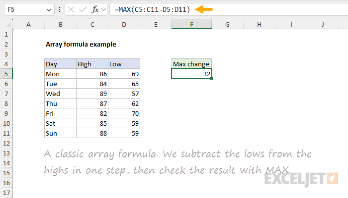
This is an array formula. Working from the inside out, we first subtract the low temps from the high temps:
C5:C11-D5:D11 // array operation
Each range contains 7 values. The subtraction runs on all 7 pairs at once, producing a new array of 7 differences:
{86;84;89;87;82;85;88}-{69;65;57;62;70;59;59}
= {17;19;32;25;12;26;29}
This is called an array operation, a calculation that runs across multiple values simultaneously. The resulting array is handed to MAX, which returns the largest value: 32.
=MAX({17;19;32;25;12;26;29}) // returns 32
That's it. The formula is easy to understand once you see how the array operation works. The key insight is that Excel can perform calculations on entire ranges at once, not just individual cells.
Array formulas can return a single result (like the MAX example above) or multiple results. In modern Excel, when a formula returns multiple results, they spill onto the worksheet automatically.
Formula: Basic array formula example
Videos: What is an array formula? | 3 basic array formulas
What are dynamic arrays?
Dynamic arrays are the biggest change to Excel formulas in years. Maybe ever. The core idea is that when a formula returns more than one value, the results spill automatically into adjacent cells on the worksheet. The cells that receive these results are called the spill range. For example, if we use the UNIQUE function to extract unique values from a list of 12 cities, UNIQUE returns an array of unique values, and those values spill into a range of cells below the formula:
=UNIQUE(B5:B16) // returns unique cities
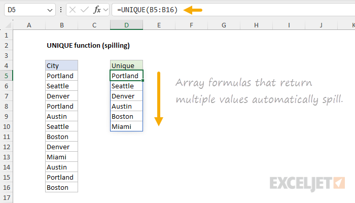
In this example, the spill range is D5:D10. When the source data changes, the spill range expands or contracts automatically. This is the idea of a dynamic array.
The spill range reference
To reference a spill range in another formula, use a hash symbol (#) after the first cell in the spill range. For example, if the UNIQUE formula above is in D5, you can count the unique cities by feeding the spill range into the COUNTA function like this:
=COUNTA(D5#) // count spilled results
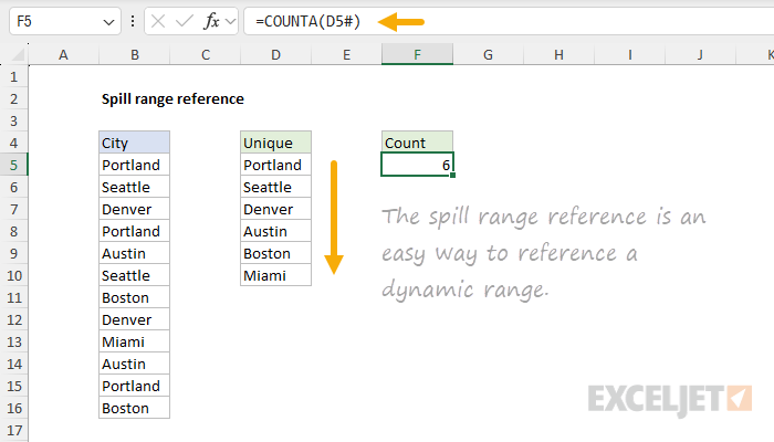
The # operator tells Excel to refer to the entire spill range, whatever its current size. The spill range reference will track the spill range as it grows or shrinks.
Note also that when you select a cell that contains a formula that spills, Excel highlights the entire spill range with a blue border. This makes it easy to verify the size of the spill range.
Native behavior
It's important to understand that dynamic array behavior is native. It's not limited to the new functions. It applies to the entire formula engine. When any formula returns multiple results, those results will spill. This includes older functions that were never designed to return multiple values.
For example, in older versions of Excel, giving the LEN function a range that contains 5 text strings would return just one result. In Dynamic Excel, LEN returns a character count for every cell in the range:
=LEN(A1:A5) // returns 5 values
Similarly, VLOOKUP can now return multiple columns by providing an array of column indexes. In the example below, VLOOKUP returns all three columns of the table. The formula in F5 looks like this:
=VLOOKUP("jose",B5:D10,{1,2,3},0) // returns 3 columns
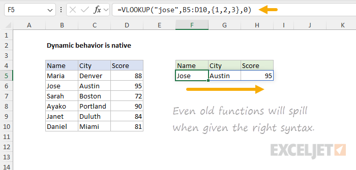
Yes, you can easily get VLOOKUP to return multiple columns by providing an array of column indexes!
Recognizing array constants
Note that in the formula above {1,2,3} is called an array constant that refers to columns 1, 2, and 3 of the table. Array constants are hard-coded values that are enclosed in curly braces.
What about Control + Shift + Enter?
In older versions of Excel (Legacy Excel), many array formulas had to be entered with Control + Shift + Enter (CSE). When entered this way, Excel would display curly braces around the formula in the formula bar:
{=MAX(C5:C11-D5:D11)} // curly braces = CSE array formula
However, if you forgot to use CSE, the formula could return an incorrect result with no warning, a silent failure that caused confusion and headaches. In modern Excel, CSE is no longer needed. Excel automatically recognizes when a formula involves an array operation and handles it correctly. Old CSE formulas still work for compatibility, but you don't need to enter new formulas this way.
Video: Spilling and the spill range | Dynamic arrays are native
Simple array formula examples
Let's look at some practical examples of array formulas using the new dynamic array functions. These are simple formulas that illustrate how arrays work in modern Excel.
Sort data
The SORT function sorts a range and spills the sorted results:
=SORT(B5:D12,3,-1) // sort by column 3, descending
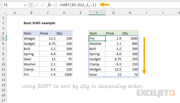
The second argument specifies which column to sort by, and the third argument controls the sort order (1 for ascending, -1 for descending).
Video: Basic sort function example
Filter data by criteria
The FILTER function extracts rows that match criteria. In the worksheet below, we are using FILTER to extract rows where the Status is "Pass":
=FILTER(B5:E15,E5:E15="pass","not found") // filter by status
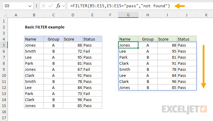
FILTER evaluates the criteria against each row. The expression E5:E15="pass" produces an array of TRUE/FALSE values, one for each row:
{TRUE;FALSE;TRUE;TRUE;FALSE;TRUE;TRUE;TRUE;FALSE;TRUE;TRUE}
FILTER returns only the rows where the result is TRUE. The third argument provides a default value if nothing matches.
Formula: Basic filter example
Video: Filter function basic example
Chaining functions together
Dynamic array functions can be nested together to perform multiple operations in one formula. For example, to extract unique values from a list and sort them:
=SORT(UNIQUE(B5:B16)) // sorted unique values
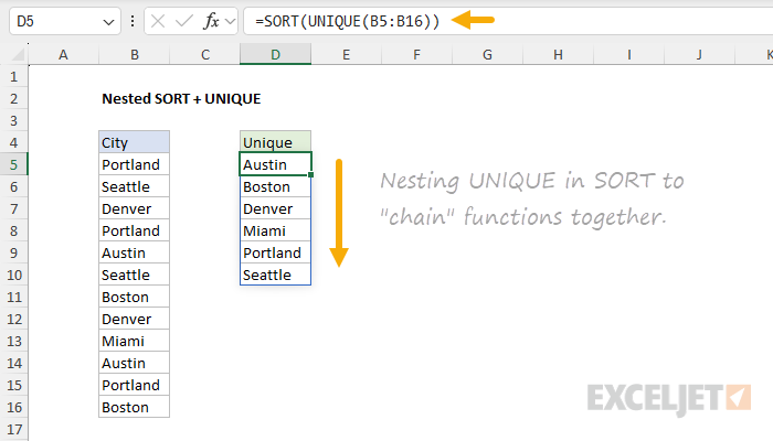
UNIQUE returns an array of unique values, and SORT takes that array and sorts it. Each function does one thing, and you can combine them to get the result you need.
Key observation: When you chain or nest functions together, you are actually "piping" arrays from one function to another. The flow is from the inner function to the outer function.
Video: Nesting dynamic array formulas
Advanced array formula examples
Once you're comfortable with the basics, array formulas open up some powerful techniques. These examples show how to combine array operations with Boolean logic and newer array functions.
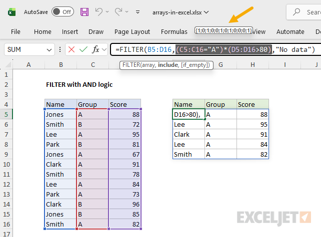
Filter with AND logic
To filter with multiple criteria using AND logic, multiply the criteria expressions together:
=FILTER(B5:D16,(C5:C16="A")*(D5:D16>80),"No data")
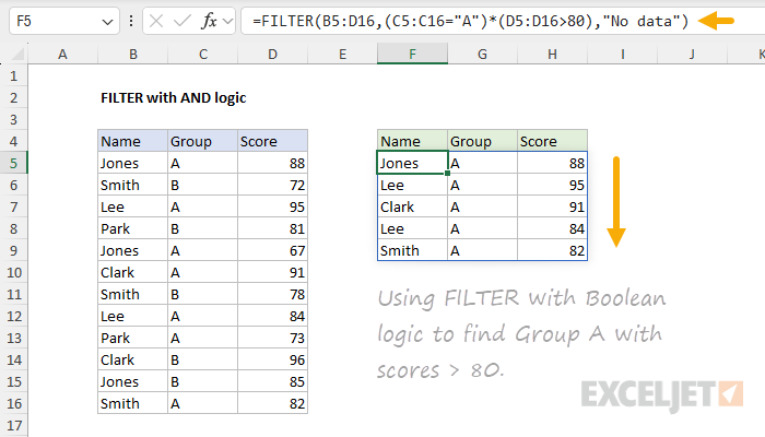
Each criteria expression returns an array of TRUE and FALSE values. When you multiply them together, Excel converts TRUE to 1 and FALSE to 0, and the multiplication acts as AND logic: a row passes through FILTER only when both criteria are met (1 * 1 = 1). Any row where either criterion fails gets a 0.
Formula: Filter with multiple criteria
Video: Filter function with two criteria | Boolean operations in array formulas
Filter with OR logic
To apply OR logic in array criteria, use addition instead of multiplication:
=FILTER(B5:D14,(C5:C14="red")+(C5:C14="pink"),B5:D14)
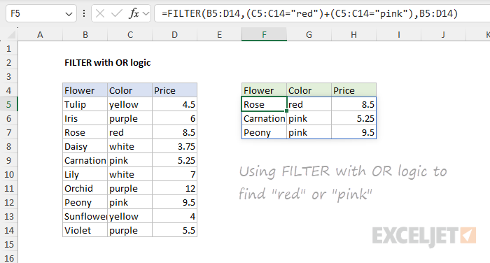
Here, addition acts as OR: a row passes through FILTER if either condition is TRUE. The expression (C5:C14="red")+(C5:C14="pink") produces an array like {0;0;1;0;1;0;0;1;0;0}, and FILTER returns all rows where the value is 1 or greater.
Video: Filter with Boolean logic | Boolean operations in array formulas
Combine data from multiple ranges
The VSTACK function combines arrays vertically. When paired with UNIQUE, it can extract unique values from multiple ranges in a single formula:
=UNIQUE(VSTACK(range1,range2,range3))
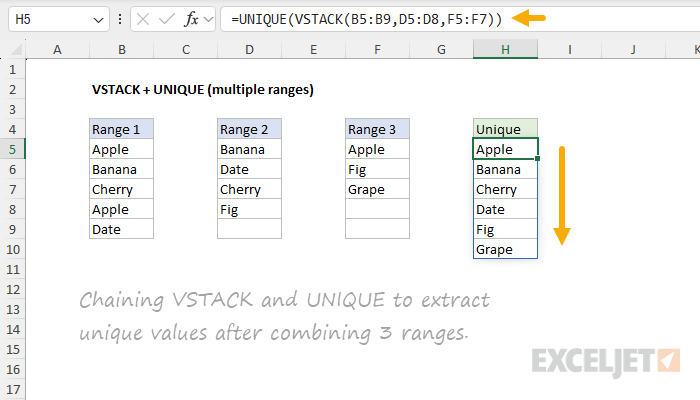
VSTACK stacks the three ranges into one array, and UNIQUE extracts the unique values from the combined result. This pattern is useful when data is spread across multiple tables or worksheets.
Formula: Unique values from multiple ranges
Random selection with TAKE, SORTBY, and RANDARRAY
This example shows how newer array functions can be combined to solve non-trivial problems. In the example below, the goal is to randomly select 3 names from a list of 12. The formula in cell D5 is:
=TAKE(SORTBY(B5:B16,RANDARRAY(ROWS(B5:B16))),3)
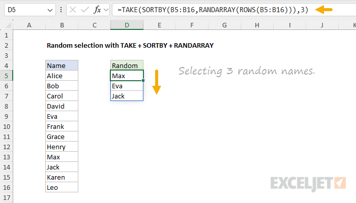
Working from the inside out:
ROWS(B5:B16)returns 12 (the number of names)RANDARRAY(12)generates 12 random numbersSORTBY(B5:B16,...)sorts the names by the random numbers (shuffles them)TAKE(...,3)returns the first 3 from the shuffled list
Each of the four functions does one simple job. When combined together, they solve a problem that would have been very difficult with traditional formulas.
Formula: Random list of names
RANDARRAY is a volatile function that will recalculate with each worksheet change. If you need a stable random result, see this article.
Arrays and ranges not always interchangeable
I mentioned earlier that a range like B5:B10 is just a vertical array of values. That's true, but the relationship only goes one direction. The *IFS family of functions (SUMIFS, COUNTIFS, AVERAGEIFS, MAXIFS, MINIFS, etc.) requires actual cell ranges for their range arguments. They will not accept in-memory arrays returned by other functions. For example, suppose you want to count a list of dates by year to see how many occur in 2026. You might try feeding the YEAR function directly into COUNTIFS like this:
=COUNTIFS(YEAR(B5:B16),2026) // won't work
The idea is perfectly logical, but Excel will reject this formula with a "There's a problem with your formula" error. The problem is that COUNTIFS requires a range for its first argument, an actual reference to cells on the worksheet. The formula YEAR(B5:B16) returns an in-memory array, which is not the same thing. This limitation exists because functions like SUMIFS and COUNTIFS predate dynamic arrays and were designed for range references only. Most other functions in Excel will accept arrays without trouble.
One workaround is to use SUM or SUMPRODUCT like this:
=SUM(--(YEAR(B5:B16)=E5)) // works in modern Excel
=SUMPRODUCT(--(YEAR(B5:B16)=E5)) // works in all versions
The comparison returns an array of TRUE and FALSE values, and the double negative (--) converts these values into an array of 1s and 0s. The SUM or SUMPRODUCT function then returns the sum of the array.
How to inspect arrays in Excel
When working with array formulas, it's very helpful to see the intermediate arrays that a formula produces. There are four good ways to do this in Excel. Let's take a look at each, from the newest to the most traditional.
Select to preview (Excel 365)
In recent versions of Excel 365, you can inspect any part of a formula simply by selecting it while in edit mode. When you select an expression, Excel displays the evaluated result, including arrays, in a tooltip near the formula bar. This is a nice way to inspect arrays because it's non-destructive: the formula is not modified in any way.
The F9 key
The traditional way to inspect arrays is with the F9 key. While editing a formula, select any expression and press F9. Excel replaces the selected expression with the evaluated result. For example, selecting C5:C11-D5:D11 and pressing F9 might show an array like this:
{17;19;32;25;12;26;29}
In the worksheet below, we have selected the include argument, (C5:C16="A")*(D5:D16>80), of this formula and pressed F9 to see the evaluated result:
=FILTER(B5:D16,(C5:C16="A")*(D5:D16>80),"No data")
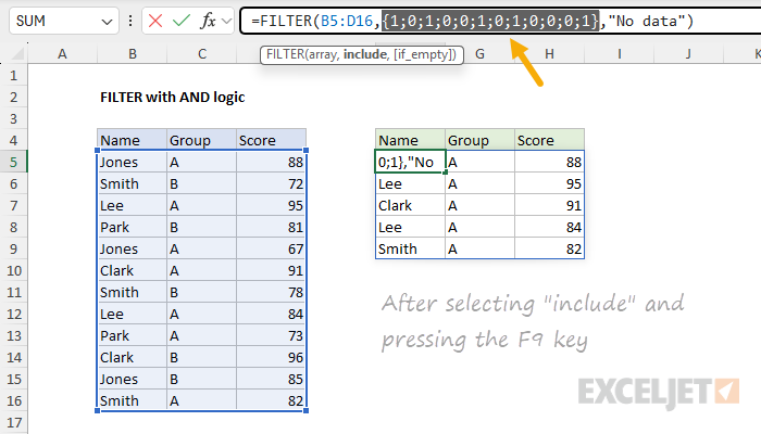
This lets you see exactly what an array operation produces. One important caution: pressing F9 replaces the expression with literal values in the formula bar. Press Escape to undo the change and restore the original formula. If you press Enter, the literal values will be saved in the formula.
The best way to select arguments quickly in a formula is to use the function screen tip window that shows up when you click into a formula. Just click a named argument and that part of the formula will be selected for you.
Evaluate Formula dialog
Excel's Evaluate Formula tool (Formulas tab > Evaluate Formula) lets you step through a formula one expression at a time. Each click evaluates the next part of the formula, showing intermediate results including arrays. This is especially useful for complex formulas where you want to see the evaluation order.
ARRAYTOTEXT
The ARRAYTOTEXT function converts an array to a text string, letting you see the values on the worksheet. With the second argument set to 1 (strict format), it shows the array exactly as Excel sees it, with semicolons separating rows and commas separating columns:
=ARRAYTOTEXT(B5:B10,1) // {"Portland";"Seattle";"Denver";"Austin";"Boston";"Miami"}
This is handy when you want a persistent and dynamic representation of an array rather than a temporary view with F9 or select to preview.
New functions for working with arrays
Excel has introduced many new functions that work directly with arrays. Here's an overview, organized by category.
Dynamic array functions
The first wave of dynamic array functions arrived with the introduction of the dynamic array engine. These functions return arrays that spill onto the worksheet:
| Function | Purpose |
|---|---|
| FILTER | Filter data and return matching records |
| SORT | Sort range by column |
| SORTBY | Sort range by another range or array |
| UNIQUE | Extract unique values from a list or range |
| SEQUENCE | Generate an array of sequential numbers |
| RANDARRAY | Generate an array of random numbers |
Video: New dynamic array functions in Excel
Array reshaping and manipulation
These newer functions let you reshape, combine, and extract portions of arrays:
| Function | Purpose |
|---|---|
| VSTACK | Stack arrays vertically |
| HSTACK | Stack arrays horizontally |
| TOCOL | Convert array to a single column |
| TOROW | Convert array to a single row |
| WRAPCOLS | Wrap a row array into columns |
| WRAPROWS | Wrap a row array into rows |
| TAKE | Return rows/columns from the start or end of an array |
| DROP | Remove rows/columns from the start or end of an array |
| CHOOSECOLS | Return specific columns from an array |
| CHOOSEROWS | Return specific rows from an array |
| EXPAND | Expand an array to specified dimensions |
LAMBDA and helper functions
The LAMBDA function lets you create custom functions, and a set of helper functions let you apply LAMBDA across arrays:
| Function | Purpose |
|---|---|
| LAMBDA | Create a custom, reusable function |
| LET | Assign names to values and expressions |
| MAP | Apply a LAMBDA to each value in an array |
| REDUCE | Reduce an array to a single value with a LAMBDA |
| SCAN | Scan an array, returning intermediate results |
| BYCOL | Apply a LAMBDA to each column |
| BYROW | Apply a LAMBDA to each row |
| MAKEARRAY | Create an array using a LAMBDA |
Text functions
Several newer text functions are array-aware and work naturally with dynamic arrays:
| Function | Purpose |
|---|---|
| TEXTSPLIT | Split text by delimiter into an array |
| TEXTAFTER | Extract text after a delimiter |
| TEXTBEFORE | Extract text before a delimiter |
| TEXTJOIN | Join array of text values with a delimiter |
| ARRAYTOTEXT | Convert an array to a text string |
Lookup functions
The latest lookup functions were designed to work with arrays from the start:
| Function | Purpose |
|---|---|
| XLOOKUP | Modern replacement for VLOOKUP with array support |
| XMATCH | Modern replacement for MATCH with array support |
For hands-on training with dynamic array formulas, see our video course: Dynamic Array Formulas.
Summary
Arrays are no longer an advanced or optional topic in Excel. With dynamic arrays, the formula engine has been fundamentally upgraded, and arrays are much more relevant:
- Arrays are everywhere. Any formula that returns multiple values will now spill results onto the worksheet.
- Powerful new functions. Excel has added functions for filtering, sorting, extracting unique values, reshaping arrays, and much more.
- Chainable. Dynamic array functions can be nested together to solve complex problems with clean, readable formulas.
- Easy to inspect. Tools like select-to-preview and F9 let you see exactly what's happening inside an array formula.
- No more CSE. You never need to enter a formula with Control + Shift + Enter in modern Excel.
Dynamic arrays will change how you think about Excel. The new functions are faster to write, easier to understand, and much more powerful than the Excel formulas of the past.


